Mathematics for ML

In 1847, Augustin-Louis Cauchy proposed a general method to solve systems of simultaneous equations, to shorten the long computations of the orbits of celestial bodies. Instead of eliminating the unknowns one at a time, the method minimizes the sum of the squares of the equations. At each step, it moves all the unknowns at once against the partial derivatives of that sum, i.e. in the direction in which the sum decreases the fastest (Cauchy and the Gradient Method). This was gradient descent. Today, linear algebra, calculus and optimization are the mathematics behind most machine learning models. Their data and parameters are vectors and matrices, and their training follows the gradient of a loss function towards a minimum, as Cauchy’s method did.

This post is a brief summary of the topics in mathematics that are relevant to ML engineers on a daily basis, extracted from the books in the resources section. It covers matrices and systems of linear equations, vector spaces, linear mappings, analytic geometry, matrix decompositions, vector calculus, backpropagation and automatic differentiation, and continuous optimization.

Properties of Matrices

Matrices have the properties of associativity \((AB)C = A(BC)\) and distributivity \((A+B)C = AC + BC\) and \(A(B+C)=AB+AC\). Unlike the product of numbers, the matrix product is not commutative: in general, \(AB \neq BA\). There is no division operator defined between matrices, as \(AB^{-1}\) and \(B^{-1}A\) usually differ. The equivalent is multiplication by the inverse (when it exists), e.g. \(A/B = AB^{-1}\).

Inverse: not every matrix \(A\) has an inverse \(A^{-1}\). If it exists, \(A\) is called regular/invertible/non-singular. Otherwise, it is called singular/non-invertible. The inverse satisfies \(AA^{-1} = I = A^{-1}A\) and \((AB)^{-1}=B^{-1}A^{-1}\), and two matrices \(A\) and \(B\) are inverses of each other if \(AB=I=BA\).

Transpose: \({(A^{\intercal})^{\intercal}}=A\), \((A+B)^{\intercal}=A^{\intercal}+B^{\intercal}\), \((AB)^{\intercal}=B^{\intercal}A^{\intercal}\).

Symmetric iff \(A=A^{\intercal}\). Thus, \(A\) is square. Also, if \(A\) is invertible, then \(A^{\intercal}\) is also invertible and \((A^{\intercal})^{-1}=(A^{-1})^{\intercal}\). The sum of symmetric matrices is a symmetric matrix, but the product of symmetric matrices usually is not.

Systems of Linear Equations

A System of Linear Equations (SLE) with equations of the type \(a_1x_1 + ...+ a_nx_n = b\), for constants \(a_1\) to \(a_n\) and \(b\) and unknown \(x\), can be written as \(A x=b\). The general solution of an SLE is found analytically or with Gaussian Elimination of the augmented matrix \([A \mid b]\), i.e. the matrix \(A\) with the vector \(b\) as an extra column.

In a geometric representation, the solution is the intersection of all the lines (or hyperplanes, in higher dimensions) defined by the different equations. Thus, such a system can have no solution, exactly one, or infinitely many solutions, as two lines in the plane are parallel, cross at one point, or are the same line. There are infinitely many solutions e.g. when there are more unknowns than equations and a solution exists. When no solution exists for \(Ax=b\), one has to resort to approximate solutions.

Analytically, when \(A\) is square and invertible, the solution for \(Ax=b\) is \(x=A^{-1}b\). Otherwise, e.g. when there are more equations than unknowns, the system usually has no solution. The approximate solution is then the \(x\) that minimizes the squared error \(\Vert Ax - b \Vert^2\), the solution of the least squares problem. Setting the derivative of the squared error with respect to \(x\) to zero gives the normal equations \(A^{\intercal} Ax = A^{\intercal}b\) and, when \(A^{\intercal}A\) is invertible:

\[x = (A^{\intercal}A)^{−1}A^{\intercal}b\]

\((A^{\intercal}A)^{−1}A^{\intercal}\) is called the pseudo-inverse of \(A\), which can be computed for non-square matrices \(A\). It only requires that \(A^{\intercal}A\) is positive definite, which is the case iff \(A\) has full column rank (both terms are defined below). With \(\hat{x}\) the solution above, \(x\) the true value, and \(b = Ax + \varepsilon\) for a zero-mean noise \(\varepsilon\), the least squares solution is unbiased:

\[\mathbb{E}[\hat{x}] = (A^{\intercal}A)^{−1}A^{\intercal} \, \mathbb{E}[b] = (A^{\intercal}A)^{−1}A^{\intercal}(Ax) = x\]

Let \(A^{+}=(A^{\intercal}A)^{−1}A^{\intercal}\). Then:

\[\operatorname{Var}[\hat{x}] = \operatorname{Var}[A^{+}b] = A^{+} \, \operatorname{Var}[b] \, (A^{+})^{\intercal} = \sigma^2 A^{+} (A^{+})^{\intercal} = \sigma^2 \, (A^{\intercal}A)^{−1}A^{\intercal} \, A (A^{\intercal}A)^{-1} = \sigma^2 \, (A^{\intercal}A)^{−1}\]

The derivation uses \(\operatorname{Var}[A^{+}b] = A^{+} \, \operatorname{Var}[b] \, (A^{+})^{\intercal}\) (formula 375 in The Matrix Cookbook), \((A^{+})^{\intercal} = A (A^{\intercal}A)^{-1}\) (as \(A^{\intercal}A\) is symmetric) and \(A^{\intercal} \, A (A^{\intercal}A)^{-1}=I\), and assumes uncorrelated noise with equal variance, i.e. \(\operatorname{Var}[b] = \sigma^2 I\).

With Gaussian Elimination on \([A \mid b]\), the forward pass puts the matrix in Row-Echelon form, i.e. a staircase structure, from which the unknowns are found from the last row up (back substitution). A row-echelon matrix is in reduced row-echelon form if the leading entry of each row (the pivot) is 1 and the pivot is the only nonzero entry in its column.

The inverse is computed by finding the matrix \(X\) that satisfies \(AX=I\), so that \(X=A^{-1}\). Gaussian Elimination is used to solve the SLE \([A \mid I]\) and turn it into \([I \mid A^{-1}]\).

Gaussian Elimination has a cubic computational complexity: it takes about \(2n^3/3\) arithmetic operations for \(n\) equations. In matrix form, its forward pass factors \(A\) into a lower and an upper triangular matrix, \(A = LU\) (the LU decomposition), which is how computers usually solve dense systems. Large dense systems are still solved this way. The HPL benchmark, which ranks the TOP500 supercomputers, solves a dense system with an LU decomposition. El Capitan, the first of the list of November 2025, solved a system of 24,768,000 unknowns in about an hour and a half: about \(10^{22}\) operations, at \(1.8 \times 10^{18}\) operations per second (TOP500).

Large sparse systems, such as those of discretized differential equations, are solved iteratively instead, e.g. with the Jacobi or Gauss-Seidel methods, as each iteration only multiplies the sparse matrix by a vector. The main idea is: to solve \(Ax=b\) iteratively, one sets up an iteration of the form \(x^{(k+1)} = Cx^{(k)} + d\), with suitable \(C\) and \(d\), that reduces the error \(\Vert x^{(k+1)}-x_* \Vert\) in every iteration and converges to the solution \(x_*\). Jacobi computes all entries of \(x^{(k+1)}\) in parallel from \(x^{(k)}\), while Gauss-Seidel uses each new entry as soon as it is computed, which often converges faster but is sequential.

Vector Spaces

A vector space \(V\) is a set of elements, the vectors, that can be added together and multiplied by scalars, with results that stay in \(V\), e.g. \(\mathbb{R}^n\). A non-empty subset \(U ⊆ V\) that is closed under these two operations is itself a vector space, a subspace of \(V\), e.g. a line or a plane through the origin of \(\mathbb{R}^3\).

A norm assigns each vector \(x\) a length \(\Vert x \Vert \ge 0\) that is zero only for \(x = 0\), scales with the vector, \(\Vert \lambda x \Vert = \vert \lambda \vert \, \Vert x \Vert\), and satisfies the triangle inequality \(\Vert x + y \Vert \le \Vert x \Vert + \Vert y \Vert\). It is written as \(\Vert x \Vert\) or \(\vert x \vert\). Examples of norms are the Manhattan norm \(\Vert x \Vert_1 = \sum_i \vert x_i \vert\) and the Euclidean norm \(\Vert x \Vert_2 = \sqrt{\sum_i x_i^2}\).

With an inner product \(<x,y>\), such as the dot product \(x^{\intercal}y\) (both defined below), the length of a vector is \(\Vert x \Vert = \sqrt{<x,x>}\), which is the Euclidean norm \(\sqrt{x^{\intercal}x}\) for the dot product. The distance between two vectors is \(d(x,y) = \Vert x-y \Vert = \sqrt{ <x-y, x-y>}\). The Cauchy-Schwarz Inequality states that \(\vert <x, y> \vert \le \Vert x \Vert \, \Vert y \Vert\).

The term vector multiplication is not well defined. Theoretically, it could be:

an element-wise multiplication \(c_j = a_j b_j\) (the Hadamard product),
the outer product \(ab^{\intercal}\), or
the inner product, scalar product or dot product \(<a, b> = a \cdot b = a^{\intercal}b\), which has the geometric interpretation \(a \cdot b = \vert a \vert \, \vert b \vert \, \cos \, \theta\) (where \(\vert a \vert\) is the magnitude (norm) of \(a\), and \(\theta\) is the angle between \(a\) and \(b\)). Note that the dot product is defined specifically for Euclidean spaces. An inner product, on the other hand, is a notion defined for a generic vector space. The dot product is commutative: \(a \cdot b = b \cdot a\).
the cross product of two vectors in \(\mathbb{R}^3\), with the geometric interpretation \(a \times b = \vert a \vert \, \vert b \vert \, \sin \, \theta \, n\) (where \(n\) is the unit vector perpendicular to \(a\) and \(b\), given by the right-hand rule), which returns a vector instead of a scalar as in the dot product. It is not commutative, but anti-commutative: \(a \times b = -(b \times a)\).

A linear combination \(v\) of vectors \(x_1, ..., x_k\) is a sum of the scaled vectors, i.e. \(v = \sum_{i=1}^k \lambda_i x_i \in V\), for constants \(\lambda_i\). If there is a linear combination of vectors \(x_1, ..., x_k\) such that \(\sum_{i=1}^k \lambda_i x_i=0\) with at least one \(\lambda_i \neq 0\), then the vectors are linearly dependent. If only the trivial solution exists, with all \(\lambda_i=0\), then they are linearly independent.

Intuitively, a set of linearly independent vectors consists of vectors that have no redundancy, i.e. if any of those vectors is removed from the set, something is lost in the representation. To find out if a set of vectors is linearly independent, write all vectors as columns of a matrix and perform the forward pass of Gaussian Elimination, i.e. until the row-echelon form. All column vectors are linearly independent iff all columns are pivot columns. Otherwise, every column without a pivot can be expressed as a linear combination of the pivot columns (as these form a basis of that vector space).

For a given vector space \(V\), if every vector can be expressed as a linear combination of a set of vectors \(A=\{ x_1, ..., x_n\}\), then \(A\) is a generating set of \(V\). The set of all linear combinations of \(A\) is called the span of \(A\). Moreover, \(A\) is called minimal if there exists no smaller set that spans \(V\). Every linearly independent generating set of \(V\) is minimal and is called a basis of \(V\).

A basis is a minimal generating set and a maximal linearly independent set of vectors. All the bases of a vector space have the same number of vectors, its dimension: e.g. the standard basis \(e_1, ..., e_n\) of \(\mathbb{R}^n\), where \(e_i\) has a 1 in entry \(i\) and zeros elsewhere, has \(n\) vectors. A basis of a vector space \(U\) can be found from the row-echelon form of a matrix with the spanning vectors of \(U\) as columns. The spanning vectors in the pivot columns are a basis of \(U\).

The rank of a matrix is the number of its linearly independent columns, i.e. the dimension of its column space (the span of its columns). A fundamental result of linear algebra is that the rank is also the number of linearly independent rows, so that \(rk(A)=rk(A^{\intercal})\). A matrix \(A \in \mathbb{R}^{n \times n}\) is invertible iff \(rk(A)=n\), and an SLE \(Ax=b\) can only be solved if \(rk(A) = rk (A \mid b)\). A matrix has full rank if its rank equals the largest possible rank for a matrix of its dimensions, the smaller of its numbers of rows and columns, otherwise it is rank deficient. A matrix whose rank equals its number of columns has full column rank.

Linear Mapping

A Linear Mapping (a.k.a. linear transformation or map) is a function \(\Phi: V \rightarrow W\) for vector spaces \(V\), \(W\), such that \(\Phi (\lambda x + \psi y) = \lambda \Phi(x) + \psi \Phi(y)\), for constants \(\lambda, \psi\) and \(x, y \in V\). In other words, it maps sums of vectors to sums and scaled vectors to scaled vectors, as a rotation or a scaling of the plane does. It can also be represented as a matrix (not only as a function).

\(\Phi\) is called injective if \(\Phi(x)=\Phi(y) \rightarrow x = y\); \(\,\,\) surjective if \(\Phi(V)=W\); \(\,\,\) bijective if both. Surjective means that every element in \(W\) can be reached from \(V\). Bijective means the mapping can be undone, i.e. there is a mapping \(\Psi : W \rightarrow V\) such that \(\Psi \circ \Phi(x) = x\) and \(\Phi \circ \Psi(y) = y\). Special cases:

Isomorphism \(\Phi: V \rightarrow W\) if linear and bijective. Finite-dimensional vector spaces \(V\) and \(W\) are isomorphic iff \(dim(V) = dim(W)\), i.e. there exists a linear, bijective mapping between any two vector spaces of the same dimension;
Endomorphism \(\Phi : V \rightarrow V\) if linear;
Automorphism \(\Phi : V \rightarrow V\) if linear and bijective.

For linear mappings \(Φ : V → W\) and \(Ψ : W → X\), the mapping \(Ψ ◦ Φ : V → X\) is also linear. If \(Φ : V → W\) is an isomorphism, then \(Φ^{−1} : W → V\) is an isomorphism, too.

For \(y=Ax\), where \(x\) is a set of coordinates, \(A\) is the transformation matrix of \(x\) into the new coordinates \(y\), i.e. a transformation matrix can be used to map coordinates from one ordered basis into another ordered basis.

Two matrices \(A, B \in \mathbb{R}^{m \times n}\) are equivalent if there exist regular matrices \(S \in \mathbb{R}^{n \times n}\) and \(T \in \mathbb{R}^{m \times m}\), such that \(B = T^{-1}A S\), i.e. the matrices can be transformed into one another by a combination of elementary row and column operations. Two matrices \(A, B \in \mathbb{R}^{n \times n}\) are similar if there exists a regular matrix \(S \in \mathbb{R}^{n \times n}\), such that \(B = S^{-1}A S\). Thus, similar matrices are always equivalent, but not the other way around.

For \(\Phi : V \rightarrow W\), the kernel is the set of vectors \(v \in V\) that \(\Phi\) maps onto the neutral element \(0_W \in W\), i.e. \(\{ v \in V : \Phi(v)=0_W \}\). The kernel space (\(ker\) or null space, a subspace of the domain) of a linear mapping is the solution set of the SLE \(Ax=0\), i.e. it captures all possible linear combinations of the elements in \(\mathbb{R}^n\) that produce \(0\). The image (\(Im\), a subspace of the codomain) of a linear mapping is the set of vectors \(w \in W\) that can be reached by \(Φ : V → W\) from any vector in \(V\). For a linear mapping \(Φ : V →W\), it holds that \(\,\,ker(Φ) \subseteq V\) and \(Im(Φ) \subseteq W\).

The Rank-Nullity theorem states that \(dim(ker(Φ)) + dim(Im(Φ)) = dim(V)\), for vector spaces \(V\), \(W\) and a linear mapping \(Φ : V →W\). As an example, the mapping \((x_1, x_2, x_3) \mapsto (x_1, x_2, 0)\) of \(\mathbb{R}^3\) has a kernel of dimension 1 (the \(x_3\) axis, which it maps to \(0\)) and an image of dimension 2 (the plane \(x_3 = 0\)), and \(1 + 2 = 3\).

An affine mapping / transformation is a linear transformation followed by a translation, and can define translation, scaling, rotation and shearing. Affine transformations keep the structure invariant, and preserve parallelism and dimension.

Analytic Geometry

A bilinear mapping \(\Omega : V \times V \rightarrow \mathbb{R}\) is called symmetric if the order of the arguments does not matter for the final result, and positive definite if \(∀x \in V \setminus \{0\} : Ω(x, x) > 0 , Ω(0, 0) = 0\).

A symmetric matrix \(A\) is called symmetric, positive definite (s.p.d.), or positive definite for short, iff it satisfies \(∀x ∈ V\setminus \{0\} : x^{\intercal}Ax > 0\). If only \(\ge\) holds, it is instead positive semidefinite. Loosely speaking, positive definite matrices are the matrix analogues of positive numbers. For example, the covariance matrix is positive semidefinite.

A symmetric, positive definite, bilinear mapping \(\Omega : V \times V \rightarrow \mathbb{R}\) is called an inner product on \(V\) and is typically written as \(<x,y>\). If \(A\) is s.p.d., then \(<x,y> = \hat{x}^{\intercal}A\hat{y}\) defines an inner product, where \(\hat{x}, \hat{y}\) are the coordinate representations of \(x, y \in V\). The following holds if \(A \in \mathbb{R}^{n \times n}\) is s.p.d.:

the null space (kernel) of \(A\) contains only \(0\) because \(x^{\intercal} A x \gt 0\) for all \(x \neq 0\). This implies \(Ax \neq 0\) if \(x \neq 0\);
the diagonal elements \(a_{ii}\) of \(A\) are positive because \(a_{ii} = e^{\intercal}_i A e_i > 0\), where \(e_i\) is the \(i\)-th vector of the standard basis in \(\mathbb{R}^n\).

In optimization, quadratic forms \(x^{\intercal}Ax\) of positive definite matrices are always positive for non-zero \(x\) and are convex: their graph is a bowl with its minimum at \(x = 0\), as the parabola \(x^2\) in one dimension.

A metric is a function \(d:V ×V → \mathbb{R}\) where \((x, y) → d(x, y)\) satisfies the following:

\(d\) is positive definite, i.e. \(d(x, y) ⩾ 0\) for all \(x, y ∈ V\) and \(d(x, y) = 0 \Leftrightarrow x = y\);
\(d\) is symmetric, i.e. \(d(x, y) = d(y, x)\) for all \(x, y ∈ V\);
triangle inequality: \(d(x, z) ⩽ d(x, y) + d(y, z)\) for all \(x, y, z ∈ V\).

The angle \(\theta\) between two vectors is computed as \(\cos \theta = \frac{<x,y>}{\|x\| \|y\|}\), where \(<x,y>\) is typically the dot product \(x^{\intercal}y\). Thus:

\[\cos \theta = \frac{<x,y>}{\sqrt{<x,x> <y,y>}} = \frac{x^{\intercal}y}{\sqrt{x^{\intercal}xy^{\intercal}y}}\]

If \(<x,y>=0\), both vectors are orthogonal, and this is written as \(x \perp y\) (\(x\) and \(y\) are perpendicular). If, in addition, \(\|x\|=\|y\|=1\), they are orthonormal.

A square matrix \(A\) is an orthogonal matrix iff its columns are orthonormal, so that \(AA^{\intercal} = I = A^{\intercal}A\), which implies \(A^{-1}=A^{\intercal}\). An orthogonal matrix preserves lengths, as \(\Vert Ax \Vert^2 = x^{\intercal}A^{\intercal}Ax = x^{\intercal}x = \Vert x \Vert^2\), and angles: it is a rotation, possibly combined with a reflection.

The inner product of two functions \(u : \mathbb{R} \rightarrow \mathbb{R}\) and \(v: \mathbb{R} \rightarrow \mathbb{R}\) is defined as \(<u,v> = \int_a^b u(x) v(x) dx\) for lower and upper limits \(a, b < \infty\).

Let \(V\) be a vector space and \(U ⊆ V\) a subspace of \(V\). A linear mapping \(π : V → U\) is called a projection if \(π^2 = π ◦ π = π\), i.e. \(\pi\) is idempotent. In the case of matrices, \(P_\pi\) is a projection iff \(P_\pi^2 = P_\pi\).

Matrix Decompositions

Determinant

The determinant of a square matrix is the signed volume of the parallelepiped formed by its columns. For a \(2 \times 2\) matrix, it is the signed area of the parallelogram spanned by the two columns, given by:

\[\det \begin{bmatrix} a & b \\ c & d \end{bmatrix} = ad - bc\]

As an example, the columns of \(A = \begin{bmatrix} 2 & 1 \\ 1 & 2 \end{bmatrix}\) span a parallelogram of area \(\det(A) = 2 \cdot 2 - 1 \cdot 1 = 3\): the mapping \(x \mapsto Ax\) multiplies all areas by 3. The sign is negative when the mapping flips the orientation of space, as a reflection does. The determinant is zero when the columns are linearly dependent, as the parallelepiped is then flat. Determinant properties:

\(\det(AB) = \det(A) \det(B)\);
\(\det(A) = \det(A^{\intercal})\);
\(\det(A^{-1})=\frac{1}{\det(A)}\);
for more than 2 columns or rows: \(\det(A) = \sum_{k=1}^{n} (−1)^{k+j}a_{kj} \det(A_{k,j})\), where \(A_{k,j}\) is \(A\) without row \(k\) and column \(j\) (Laplace expansion along column \(j\)), which reduces the determinant to determinants of size \(n-1\);
Similar matrices have the same determinant;
for a diagonal (or triangular) matrix, the determinant is the product of the diagonal elements.

Thus, the determinant can also be computed as the product of the diagonal elements of the matrix in row-echelon form, a triangular matrix, when this form is obtained without scaling rows, and with a sign change for each row swap. Important: a square matrix \(A \in \mathbb{R}^{n \times n}\) is invertible iff \(\det(A) \neq 0\), i.e. iff it has full rank, \(rk(A)=n\).

Eigenvalues, eigenvectors and trace

For a square matrix \(A \in \mathbb{R}^{n \times n}\), \(λ ∈ \mathbb{R}\) is an eigenvalue of \(A\) and \(x ∈ \mathbb{R}^n \setminus \{0\}\) is a corresponding eigenvector of \(A\) if \(Ax = λx\). The mapping \(x \mapsto Ax\) thus keeps the eigenvector on its own line and scales it by its eigenvalue. The trace of a square matrix, the sum of its diagonal terms, equals the sum of its eigenvalues, and its determinant equals their product (counted with their multiplicity, complex eigenvalues included).

To determine the eigenvalues of \(A\), solve \(Ax = \lambda x\) or equivalently solve \(\det(A - \lambda I)=0\) for \(\lambda\), where \(p(\lambda) = \det(A - \lambda I)\) is called the characteristic polynomial. The equivalence holds because \((A - \lambda I)x = 0\) has a solution \(x \neq 0\) iff \(A - \lambda I\) is singular.

To determine the eigenvectors \(x_i\), solve \(Ax_i=\lambda_i x_i\) for each eigenvalue \(\lambda_i\) found previously. Eigenvectors corresponding to distinct eigenvalues are linearly independent. Therefore, eigenvectors of a matrix with \(n\) distinct eigenvalues form a basis of \(\mathbb{R}^n\). A square matrix with fewer (linearly independent) eigenvectors than its dimension is called defective.

As an example, consider again \(A = \begin{bmatrix} 2 & 1 \\ 1 & 2 \end{bmatrix}\). Its characteristic polynomial is \(p(\lambda) = (2 - \lambda)^2 - 1 = \lambda^2 - 4\lambda + 3 = (\lambda - 3)(\lambda - 1)\), so its eigenvalues are \(\lambda_1 = 3\) and \(\lambda_2 = 1\). Solving \((A - 3I)x = 0\) gives the eigenvector \(x_1 = [1, 1]^{\intercal}\), and solving \((A - I)x = 0\) gives \(x_2 = [1, -1]^{\intercal}\): \(A\) stretches space by 3 along the diagonal \(x_1\), and leaves the vectors along \(x_2\) unchanged. The trace, \(2 + 2 = 4\), is the sum of the eigenvalues, and the determinant, \(3\), their product. As \(A\) is symmetric, its two eigenvectors are orthogonal: \(x_1^{\intercal} x_2 = 0\).

Two vectors are called codirected if they point in the same direction, and collinear if they point in the same or opposite directions. All non-zero vectors collinear to an eigenvector are also eigenvectors: if \(x\) is an eigenvector of \(A\) associated with eigenvalue \(λ\), then for any \(c ∈ \mathbb{R}\setminus\{0\}\), \(cx\) is an eigenvector of \(A\) with the same eigenvalue, so eigenvectors are not unique. Moreover:

a matrix and its transpose have the same eigenvalues, but not necessarily the same eigenvectors;
symmetric, positive definite matrices (like a non-singular covariance matrix) always have positive, real eigenvalues. Their determinant, the product of the eigenvalues, is then positive, and they are therefore invertible;
given a matrix \(A \in \mathbb{R}^{m \times n}\), a symmetric positive semidefinite matrix \(S=A^{\intercal}A\) can always be obtained, as \(x^{\intercal}A^{\intercal}Ax = \Vert Ax \Vert^2 \ge 0\). If \(rk(A)=n\), then \(A^{\intercal}A\) is symmetric positive definite. By the spectral theorem, \(S\) has an orthonormal basis of eigenvectors with real eigenvalues, so it is positive definite iff all its eigenvalues are positive.

Graphical intuition: for a diagonal matrix (first row of the following picture), the directions of the two eigenvectors correspond to the canonical basis vectors, i.e. to the cardinal axes. Each axis is scaled by a factor equal to its eigenvalue. More generally, a mapping whose eigenvectors form a basis scales space along their directions:

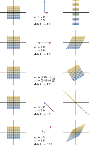
Determinants and eigenspaces. Overview of five linear mappings and their associated transformation matrices \(A_i \in \mathbb{R}^{2 \times 2}\) projecting 400 color-coded points \(x \in \mathbb{R}^2\) (left column) onto target points \(A_i x\) (right column). The central column depicts the first eigenvector (blue), stretched by its associated eigenvalue \(\lambda_1\), and the second eigenvector (red), stretched by its eigenvalue \(\lambda_2\). Each row depicts the effect of one of five transformation matrices \(A_i\) with respect to the standard basis, and gives \(\lambda_1\), \(\lambda_2\) and \(\det(A_i)\). Adapted from: Mathematics for Machine Learning, Figure 4.4

Looking at the picture, the determinant is the product of the two eigenvalues in every row, and its absolute value is the factor by which the mapping scales areas. The shear of the second row has a repeated eigenvalue and collinear eigenvectors, and the rotation of the third row has complex eigenvalues and no real eigenvectors. The mapping of the fourth row has a zero eigenvalue, so it collapses the plane onto a line, and its determinant is zero. The mapping of the last row is the matrix \(A\) of the example above divided by 2. It has the same eigenvectors, half the eigenvalues (1.5 along \([1, 1]^{\intercal}\) and 0.5 along \([1, -1]^{\intercal}\)), and a quarter of the determinant, 0.75.

Cholesky Decomposition

A symmetric, positive definite matrix \(A\) can be factorized into a product \(A = LL^{\intercal}\), where \(L\) is a lower-triangular matrix with positive diagonal elements. \(L\) is unique, and its entries can be computed one at a time, by expanding \(LL^{\intercal}\) and comparing it with \(A\). The Cholesky decomposition is used e.g. to sample from Gaussian distributions (if \(z \sim \mathcal{N}(0, I)\), then \(\mu + Lz \sim \mathcal{N}(\mu, A)\)) and to compute determinants efficiently, as \(\det(A) = \det(L) \det(L^⊤) = \det(L)^2\).

Eigendecomposition

A matrix \(A \in \mathbb{R}^{n \times n}\) is diagonalizable if it is similar to a diagonal matrix, i.e. if there is an invertible matrix \(P \in \mathbb{R}^{n \times n}\) such that \(D=P^{-1}AP\). The inverse of a diagonal matrix is obtained by replacing all diagonal elements by their reciprocals, i.e. replacing \(a_{ii}\) by \(\frac{1}{a_{ii}}\).

A matrix \(A \in \mathbb{R}^{n \times n}\) can be factored into \(A = PDP^{-1}\) iff the eigenvectors of \(A\) form a basis of \(\mathbb{R}^n\). The columns of \(P \in \mathbb{R}^{n \times n}\) are then eigenvectors of \(A\), and \(D\) is a diagonal matrix whose diagonal entries are the eigenvalues of \(A\). When this eigendecomposition (ED) exists, then:

\[\det(A) = \det(PDP^{−1}) = \det(P) \, \det(D) \, \det(P^{−1})\]

which equals \(\det(D)\), the product of the eigenvalues, and \(A^k = (PDP^{−1})^k = PD^kP^{−1}\), as each \(P^{-1}P\) in between cancels. When no eigenvalue is zero, the inverse is \(A^{-1} = PD^{-1}P^{-1}\), with the reciprocals of the eigenvalues on the diagonal of \(D^{-1}\). A symmetric matrix can always be diagonalized, with orthonormal eigenvectors (the spectral theorem), so that \(P\) is orthogonal and \(P^{-1} = P^{\intercal}\).

For the example above, \(D = \operatorname{diag}(3, 1)\), and the eigenvectors \(x_1\) and \(x_2\) are the columns of \(P = \begin{bmatrix} 1 & 1 \\ 1 & -1 \end{bmatrix}\). As both columns have length \(\sqrt{2}\), \(P^{-1} = P^{\intercal} / 2\). Powers of \(A\) are then cheap to compute, e.g. \(A^3 = P \operatorname{diag}(27, 1) P^{-1} = \begin{bmatrix} 14 & 13 \\ 13 & 14 \end{bmatrix}\), and so is its inverse, \(A^{-1} = P \operatorname{diag}(1/3, 1) P^{-1}\).

Singular Value Decomposition

The Singular Value Decomposition (SVD) is a decomposition of the form \(A = U \Sigma V^{\intercal}\):

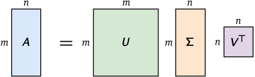
The SVD of a matrix \(A \in \mathbb{R}^{m \times n}\), \(A = U \Sigma V^{\intercal}\), with the orthogonal matrices \(U \in \mathbb{R}^{m \times m}\) and \(V \in \mathbb{R}^{n \times n}\), and \(\Sigma \in \mathbb{R}^{m \times n}\), whose only non-zero entries are the singular values on its diagonal. Adapted from: Mathematics for Machine Learning, Section 4.5

It is applicable to all matrices (not only square), and it always exists:

\(\Sigma\) is the singular value matrix, a (possibly non-square) matrix with non-negative diagonal entries \(\Sigma_{ii} = \sigma_{i} \ge 0\), and zeros elsewhere. \(\sigma_{i}\) are the singular values. \(\Sigma\) is unique. By convention, \(\sigma_{i}\) are ordered by value, with the largest at \(i=1\);
\(U\) is orthogonal and its column vectors \(u_i\) are called left-singular vectors. It is orthogonal, i.e. \(UU^{\intercal}=U^{\intercal}U=I\): its columns are orthogonal and normal (orthonormal). The left-singular vectors of \(A\) are the eigenbasis (i.e. the eigenvectors) of \(AA^{\intercal}\);
\(V\) is orthogonal and its column vectors \(v_i\) are called right-singular vectors. The right-singular vectors of \(A\) are eigenvectors of \(A^{\intercal}A\), and the singular values are the square roots of its eigenvalues, as \(A^{\intercal}A = V \Sigma^{\intercal} \Sigma V^{\intercal}\).

Computing the SVD of \(A \in \mathbb{R}^{m \times n}\) is equivalent to finding two sets of orthonormal bases \(U = (u_1,... , u_m)\) and \(V = (v_1,... , v_n)\) of the codomain \(\mathbb{R}^m\) and the domain \(\mathbb{R}^n\), respectively. From these ordered bases, the matrices \(U\) and \(V\) are constructed. The eigendecomposition of an s.p.d. matrix (\(S = S^⊤ = PDP^⊤\)) and its SVD (\(S = UΣV^⊤\)) are equivalent, by setting \(U = P = V\) and \(D = Σ\).

Matrix approximation/compression is achieved by reconstructing the original matrix using fewer singular values \(\sigma_i\). In practice, for a rank-\(k\) approximation:

\[\hat{A}(k) = \sum_{i=1}^{k} \sigma_i u_i v_i^{\intercal} = \sum_{i=1}^k \sigma_i A_i\]

where \(A_i = u_i v_i^{\intercal}\) is a matrix of rank 1, so that \(\hat{A}(k)\) needs only \(k(m+n+1)\) values instead of \(mn\). By the Eckart–Young theorem (MML book, section 4.6), no matrix of rank \(k\) is closer to \(A\) than \(\hat{A}(k)\). Its error is the first singular value left out, \(\Vert A - \hat{A}(k) \Vert_2 = \sigma_{k+1}\), in the spectral norm \(\Vert B \Vert_2\), the largest factor by which a matrix \(B\) stretches a vector (its largest singular value). The SVD and its use for image compression are illustrated below:

\(\,\,\,\,\)

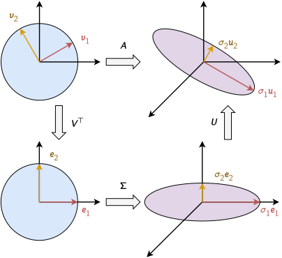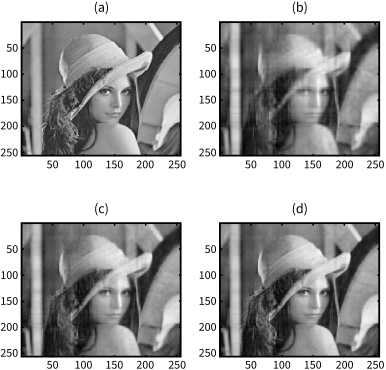
Left: the SVD of a matrix \(A \in \mathbb{R}^{3 \times 2}\) as a sequence of three transformations. Top-left to bottom-left: \(V^{\intercal}\) performs a basis change in \(\mathbb{R}^2\), which maps the right-singular vectors \(v_1\), \(v_2\) to the standard basis vectors \(e_1\), \(e_2\). Bottom-left to bottom-right: \(\Sigma\) scales by the singular values \(\sigma_1\), \(\sigma_2\) and maps from \(\mathbb{R}^2\) to \(\mathbb{R}^3\). The ellipse in the bottom-right lives in \(\mathbb{R}^3\), and the third dimension is orthogonal to the surface of the elliptical disk. Bottom-right to top-right: \(U\) performs a basis change within \(\mathbb{R}^3\), to the left-singular vectors \(u_1\), \(u_2\). Top-left to top-right: \(A = U \Sigma V^{\intercal}\) maps the unit circle directly. Right: an application of the SVD to image compression: (a) a \(256 \times 256\) gray image, and its approximations with its (b) 20, (c) 50 and (d) 85 largest singular values. Adapted from: Mathematics for Machine Learning, Figure 4.8 (left) and T. Workalemahu, Singular Value Decomposition in Image Noise Filtering and Reconstruction, Georgia State University, 2008 (right)

In the picture on the right, the approximation with 20 singular values (b) needs only 20 × (256 + 256 + 1) = 10,260 values, 16% of the 65,536 pixels of the image, but it is blurry. The approximation with 85 singular values (d) is close to the original image, but needs 43,605 values, 67% of its pixels.

Cholesky vs. Eigendecomposition vs. SVD

The SVD always exists for any matrix. The ED is only defined for square matrices and only exists if one can find a basis of eigenvectors in \(\mathbb{R}^n\), and the Cholesky decomposition only exists for s.p.d. matrices;
in SVD, domain and codomain can be vector spaces of different dimensions;
the vectors of \(P\) in ED are not necessarily orthogonal. The vectors in the matrices \(U\) and \(V\) in the SVD are orthonormal, so they do represent rotations (possibly combined with a reflection);
where it exists, the Cholesky decomposition is the cheapest: it solves a system of linear equations in about \(n^3/3\) operations, half the cost of the LU decomposition. The ED and the SVD need iterative algorithms, as the eigenvalues of a matrix larger than \(4 \times 4\) cannot be computed in a finite number of steps in general.

In practice, the ED applies to square matrices such as covariance matrices, and the SVD to any matrix, such as a data matrix with one sample per row. The Cholesky decomposition applies to s.p.d. matrices, e.g. to solve the normal equations of least squares or to sample from a Gaussian distribution. As an example, Principal Component Analysis can be computed from the ED of the covariance matrix, or from the SVD of the centered data matrix, which avoids forming the covariance matrix and is the standard approach.

Vector Calculus

Derivative

For \(h \neq 0\), the derivative of \(f\) at \(x\) is defined as the limit:

\[\frac{df}{dx} = \lim_{h \rightarrow 0} \frac{f(x+h) - f(x)}{h}\]

In the limit, the line through \((x, f(x))\) and \((x+h, f(x+h))\) becomes the tangent of \(f\) at \(x\), whose slope is the derivative.

Gradient, Jacobian and Hessian

The gradient \(\nabla_x f(x)\) of a function \(f : \mathbb{R}^n \rightarrow \mathbb{R}\) collects its \(n\) partial derivatives \(\frac{\partial f(x)}{\partial x_j}\), i.e. the derivatives with respect to one variable \(x_j\) with the others fixed. The MML book writes it as a row vector, of size \(1 \times n\), which is why the update of gradient descent below transposes it. The gradient points in the direction in which \(f\) increases the fastest. For a vector-valued function \(f : \mathbb{R}^n \rightarrow \mathbb{R}^m\), the \(m \times n\) matrix of partial derivatives \(\frac{\partial f_i(x)}{\partial x_j}\), for each function \(i\) and variable \(j\), is the Jacobian, whose rows are the gradients of the \(m\) functions. Useful rules in partial differentiation:

\[\begin{align*} & \text{Product:} & (f(x) g(x))' & = f'(x)g(x) + f(x)g'(x) \\ & \text{Quotient:} & \left(\frac{f(x)}{g(x)}\right)' & = \frac{f'(x)g(x) - f(x)g'(x)}{g(x)^2} \\ & \text{Sum:} & (f(x) + g(x))' & = f'(x)+ g'(x) \\ & \text{Chain:} & (g(f(x)))' & = (g \circ f)'(x) = g'(f(x))f'(x) = \frac{dg}{df} \frac{df}{dx} \end{align*}\]

The Hessian \(\mathbf{H}_f\) (also written \(\nabla^2 f\)) of a function \(f : \mathbb{R}^n \rightarrow \mathbb{R}\) is the collection of all second-order partial derivatives of all variables with respect to all other variables, defined by the following matrix (symmetric if the second-order partial derivatives are continuous):

\[\mathbf{H}_f = \begin{bmatrix} \dfrac{\partial^2 f}{\partial x_1^2} & \dfrac{\partial^2 f}{\partial x_1\,\partial x_2} & \cdots & \dfrac{\partial^2 f}{\partial x_1\,\partial x_n} \\[2.2ex] \dfrac{\partial^2 f}{\partial x_2\,\partial x_1} & \dfrac{\partial^2 f}{\partial x_2^2} & \cdots & \dfrac{\partial^2 f}{\partial x_2\,\partial x_n} \\[2.2ex] \vdots & \vdots & \ddots & \vdots \\[2.2ex] \dfrac{\partial^2 f}{\partial x_n\,\partial x_1} & \dfrac{\partial^2 f}{\partial x_n\,\partial x_2} & \cdots & \dfrac{\partial^2 f}{\partial x_n^2} \end{bmatrix}\]

Taylor series

The Taylor series is a representation of a function \(f\) as an infinite sum of terms that are expressed in terms of the function’s derivatives at a single point \(x_0\). The Taylor Polynomial of degree \(n\) of a function \(f\) at \(x_0\) is:

\[T_n(x) = \sum_{k=0}^n \frac{f^{(k)}(x_0)}{k!}(x-x_0)^k\]

where \(f^{(k)}\) is the \(k\)-th derivative of \(f\). The Taylor series is the Taylor polynomial of infinite order, i.e. \(T_{\infty}(x)\). If \(T_{\infty}(x)=f(x)\), the function is called analytic.

As an example, all the derivatives of \(f(x) = \exp(x)\) are \(\exp(x)\), so at \(x_0 = 0\) its Taylor polynomial is \(T_n(x) = \sum_{k=0}^n x^k / k!\), and \(T_2(0.1) = 1.105\) is close to \(\exp(0.1) = 1.10517\). For a function \(f : \mathbb{R}^d \rightarrow \mathbb{R}\) of \(d\) variables, the Taylor polynomial of degree 2 at \(x_0\) is written with the gradient and the Hessian:

\[T_2(x) = f(x_0) + \nabla_x f(x_0) \, (x - x_0) + \frac{1}{2} (x - x_0)^{\intercal} \, \mathbf{H}_f(x_0) \, (x - x_0)\]

i.e. a quadratic approximation of \(f\) around \(x_0\), which Newton’s method below uses to find a minimum.

Relevance:

in ML, it is often necessary to compute expectations, i.e. to solve integrals of the form \(\mathbb{E}[f(x)] = \int f(x) p(x) dx\). Even for parametric \(p(x)\), this integral typically cannot be solved analytically. The Taylor series expansion of \(f(x)\) is a way to find an approximate solution \(\mathbb{E}[f(x)] \approx \mathbb{E}[T_k(x)]\).
in Bayesian statistics, computing the posterior often involves integrals: \(p(x \mid y) = \frac{ p(y \mid x) p(x)}{p(y)}\), where \(p(y) = \int p(y \mid x) p(x) dx\). These integrals are often multidimensional in realistic problems and are typically analytically intractable (except in a few special cases, such as when using conjugate priors), so approximate inference must be applied, e.g. the Laplace approximation, a second-order Taylor expansion of the log-posterior around its maximum.
much of non-Bayesian statistics is based on maximum likelihood: finding the maximum of a (usually multidimensional) function, which involves knowledge of its derivatives, i.e. differentiation. Numerical methods may not be mandatory, but they are used because they are simpler (faster); it comes down to the fact that differentiation is more tractable than integration.
see Taylor expansions for the moments of functions of random variables for more details.

Newton’s method

Newton’s method (or Newton-Raphson method) is a root-finding algorithm that produces successively better approximations to the roots (or zeroes) of a real-valued function, i.e. it solves equations of the form \(f(x)=0\) by successive approximation. Iterations are defined as:

\[x_{n+1}=x_{n}-{\frac {f(x_{n})}{f'(x_{n})}}\]

The initial value \(x_0\) should be picked as close as possible to the zero. The equation of the line tangent to \(y=f(x)\) at \(x=x_0\) is then found and followed back to the \(x\) axis, which gives a new, improved guess \(x_1\).

As an example, \(\sqrt{2}\) is the positive zero of \(f(x) = x^2 - 2\), whose derivative is \(f'(x) = 2x\), so the iteration becomes \(x_{n+1} = x_n - \frac{x_n^2 - 2}{2 x_n} = \frac{1}{2} \left( x_n + \frac{2}{x_n} \right)\), the Babylonian method of computing square roots. From \(x_0 = 1\), it gives \(x_1 = 1.5\), \(x_2 = 1.41667\), \(x_3 = 1.4142157\) and \(x_4 = 1.41421356237469\), with errors of \(8.6 \times 10^{-2}\), \(2.5 \times 10^{-3}\), \(2.1 \times 10^{-6}\) and \(1.6 \times 10^{-12}\). Close to the zero, the number of correct digits about doubles at every iteration (quadratic convergence).

A stationary point of a function (a minimum, maximum or saddle point) can be found by computing the root of the derivative, i.e. \(x_{n+1}=x_{n}-{\frac {f'(x_{n})}{f''(x_{n})}}\). Each such step moves to the stationary point of the Taylor polynomial of degree 2 of \(f\) at \(x_n\), the parabola that has the same value, slope and curvature as \(f\) at \(x_n\).

For multivariate functions, the division is not defined, so it is replaced by multiplication by the inverse of the Hessian, i.e. \(x_{n+1}=x_{n}- \left(\nabla^2 f(x_{n})\right)^{-1} \left(\nabla f(x_{n})\right)^{\intercal}\), which moves to the minimum of the Taylor polynomial \(T_2\) at \(x_n\) when the Hessian is positive definite. Close to a minimum, Newton’s method needs fewer iterations than gradient descent, as it uses the curvature of the function. However, as the Hessian of a function of \(d\) variables takes \(O(d^2)\) memory and its inversion \(O(d^3)\) operations, large neural networks are trained with gradient descent instead. For \(d = 10^9\) parameters, the Hessian has \(10^{18}\) entries, 4 exabytes in FP32. The root-finding iterations are illustrated in the following animation:

Newton’s method: the tangent of \(f\) at each guess crosses the \(x\) axis at the next, improved guess, and the guesses converge to the zero of \(f\). The animation numbers the initial guess \(x_1\) (the text’s \(x_0\)), and its legend reads "Funktion" (the function \(f\)) and "Tangente" (the tangent). Source: Newton’s method

Backpropagation and Automatic Differentiation

The output \(y\) of a deep neural network (DNN) of \(K\) layers \(f_1, ..., f_K\) is computed as the composition of its layers:

\[y = (f_K ◦ f_{K−1} ◦ ... ◦ f_1)(x) = f_K(f_{K−1}( ... (f_1(x)) ... ))\]

The chain rule allows the partial derivatives to be described as follows:

\[\begin{align*} \frac{\partial L}{\partial \boldsymbol{\theta}_{K-1}} & = \frac{\partial L}{\partial \boldsymbol{f}_K} {\color{#0000FF} \frac{\partial \boldsymbol{f}_K}{\partial \boldsymbol{\theta}_{K-1}}} \\ \frac{\partial L}{\partial \boldsymbol{\theta}_{K-2}} & = \frac{\partial L}{\partial \boldsymbol{f}_K} \boxed{ {\color{#FF7300} \frac{\partial \boldsymbol{f}_K}{\partial \boldsymbol{f}_{K-1}}} {\color{#0000FF} \frac{\partial \boldsymbol{f}_{K-1}}{\partial \boldsymbol{\theta}_{K-2}}} } \\ \frac{\partial L}{\partial \boldsymbol{\theta}_{K-3}} & = \frac{\partial L}{\partial \boldsymbol{f}_K} {\color{#FF7300} \frac{\partial \boldsymbol{f}_K}{\partial \boldsymbol{f}_{K-1}}} \boxed{ {\color{#FF7300} \frac{\partial \boldsymbol{f}_{K-1}}{\partial \boldsymbol{f}_{K-2}}} {\color{#0000FF} \frac{\partial \boldsymbol{f}_{K-2}}{\partial \boldsymbol{\theta}_{K-3}}} } \\ \frac{\partial L}{\partial \boldsymbol{\theta}_i} & = \frac{\partial L}{\partial \boldsymbol{f}_K} {\color{#FF7300} \frac{\partial \boldsymbol{f}_K}{\partial \boldsymbol{f}_{K-1}}} \cdots \boxed{ {\color{#FF7300} \frac{\partial \boldsymbol{f}_{i+2}}{\partial \boldsymbol{f}_{i+1}}} {\color{#0000FF} \frac{\partial \boldsymbol{f}_{i+1}}{\partial \boldsymbol{\theta}_i}} } \end{align*}\]

where \(L\) is the loss and \(\boldsymbol{\theta}_i\) are the parameters of the layer \(\boldsymbol{f}_{i+1}\). The orange terms are partial derivatives of a layer with respect to its inputs, and the blue terms are partial derivatives of a layer with respect to its parameters. The boxed terms are the only new terms of each line; the rest is reused from the line above.

Backpropagation is a special case of the automatic differentiation algorithm, a technique to evaluate the gradient of a function by working with intermediate variables and dependencies and applying the chain rule. As an example, consider the function

\[f(x) = \sqrt{x^2 + \exp(x^2)} + \cos\left(x^2 + \exp(x^2)\right) \, .\]

By application of the chain rule, and noting that differentiation is linear, the gradient is computed as

\[\begin{align*} \frac{\mathrm{d}f}{\mathrm{d}x} & = \frac{2x + 2x \exp(x^2)}{2 \sqrt{x^2 + \exp(x^2)}} - \sin\left(x^2 + \exp(x^2)\right) \left(2x + 2x \exp(x^2)\right) \\ & = 2x \left( \frac{1}{2 \sqrt{x^2 + \exp(x^2)}} - \sin\left(x^2 + \exp(x^2)\right) \right) \left(1 + \exp(x^2)\right) \, . \end{align*}\]

As the Mathematics for Machine Learning book notes in section 5.6, where this example comes from:

Writing out the gradient in this explicit way is often impractical since it often results in a very lengthy expression for a derivative. In practice, it means that, if we are not careful, the implementation of the gradient could be significantly more expensive than computing the function, which imposes unnecessary overhead.

If the automatic differentiation algorithm is used instead, the forward pass can be done efficiently by reusing intermediate results, and the backpropagation algorithm can be broken into partial derivatives that propagate backwards through the graph.

If the function \(f\) above were implemented on a computer, some computation could be saved by using intermediate variables:

\[\begin{align*} a & = x^2 \, , \\ b & = \exp(a) \, , \\ c & = a + b \, , \\ d & = \sqrt{c} \, , \\ e & = \cos(c) \, , \\ f & = d + e \, . \end{align*}\]

The following picture illustrates the resulting computation graph, where each variable is computed from the variables on its incoming arrows:

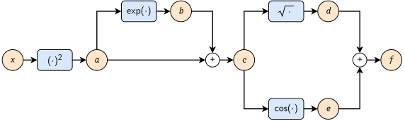
Computation graph of \(f(x) = \sqrt{x^2 + \exp(x^2)} + \cos(x^2 + \exp(x^2))\), with the intermediate variables \(a = x^2\), \(b = \exp(a)\), \(c = a + b\), \(d = \sqrt{c}\) and \(e = \cos(c)\), and \(f = d + e\). Adapted from: Mathematics for Machine Learning, Example 5.14

This is the same kind of thinking process that occurs when applying the chain rule. Note that the preceding set of equations requires fewer operations than a direct implementation of the function \(f(x)\).

The backward pass then computes the derivative of the output with respect to each variable, from \(f\) back to \(x\). Each step needs only the derivatives of the elementary operations with respect to their inputs:

\[\frac{\partial a}{\partial x} = 2x, \quad \frac{\partial b}{\partial a} = \exp(a), \quad \frac{\partial c}{\partial a} = 1 = \frac{\partial c}{\partial b}, \quad \frac{\partial d}{\partial c} = \frac{1}{2\sqrt{c}}, \quad \frac{\partial e}{\partial c} = -\sin(c), \quad \frac{\partial f}{\partial d} = 1 = \frac{\partial f}{\partial e}\]

Following the arrows of the graph backwards, the chain rule sums the contributions of all the paths that leave a variable:

\[\begin{align*} \frac{\partial f}{\partial c} & = \frac{\partial f}{\partial d} \frac{\partial d}{\partial c} + \frac{\partial f}{\partial e} \frac{\partial e}{\partial c} \, , \\ \frac{\partial f}{\partial b} & = \frac{\partial f}{\partial c} \frac{\partial c}{\partial b} \, , \\ \frac{\partial f}{\partial a} & = \frac{\partial f}{\partial b} \frac{\partial b}{\partial a} + \frac{\partial f}{\partial c} \frac{\partial c}{\partial a} \, , \\ \frac{\partial f}{\partial x} & = \frac{\partial f}{\partial a} \frac{\partial a}{\partial x} \, . \end{align*}\]

As an example, at \(x = 1\) the forward pass computes \(a = 1\), \(b = \exp(1) = 2.718\), \(c = 3.718\), \(d = 1.928\), \(e = -0.838\) and \(f = 1.090\). The backward pass then gives \(\partial f / \partial c = 1/(2d) - \sin(c) = 0.805\), \(\partial f / \partial b = \partial f / \partial c = 0.805\), \(\partial f / \partial a = b \, \partial f / \partial b + \partial f / \partial c = 2.992\) and \(\partial f / \partial x = 2x \, \partial f / \partial a = 5.98\), the value of the closed-form derivative above at \(x = 1\). Each step of the backward pass costs a few operations, so the derivative costs about as much as the function itself.

This backward pass is the reverse mode of automatic differentiation. One pass from the output back to the inputs gives the derivatives of the output with respect to all the inputs, at a small constant factor of the cost of the function. The forward mode propagates the derivatives from one input to all the outputs instead, so it needs one pass per input. A neural network has millions of parameters and one scalar loss, so it is trained with the reverse mode, of which backpropagation is the special case for neural networks.

Continuous Optimization

Training a machine learning model means finding the parameters that minimize a loss function. To check whether a stationary point is a minimum or maximum of a function, one needs to check if the second derivative is positive or negative at that point. Thus, \(\frac{d^2f(x)}{dx^2}\) is computed and evaluated at all stationary points: if \(f′′(x)>0\), the function is concave up and that point is a minimum. If \(<0\), it is concave down, and the point is a maximum; if it is zero, the test is inconclusive.

For a function of several variables, the Hessian at the stationary point plays the role of the second derivative: the point is a minimum if the Hessian is positive definite (all its eigenvalues are positive), a maximum if it is negative definite (all negative), and a saddle point if it has both positive and negative eigenvalues. With a zero eigenvalue, the test is inconclusive. As an example, \(f(x) = x_1^2 - x_2^2\) has a stationary point at \(x = 0\), with the Hessian \(\begin{bmatrix} 2 & 0 \\ 0 & -2 \end{bmatrix}\): a saddle point, which is a minimum along \(x_1\) and a maximum along \(x_2\).

Convex sets and functions

Convex sets are sets such that a straight line connecting any two elements of the set lies inside the set. Similarly, a convex function is a function where any line segment between any two distinct points on the graph of the function lies on or above the graph between the two points, i.e. \(f(\theta x + (1-\theta) y) \le \theta f(x) + (1-\theta) f(y)\) for all \(x\), \(y\) and \(\theta \in [0, 1]\).

A convex function is concave up, therefore its second derivative (if it is twice differentiable) is non-negative on its entire domain. For a function of several variables, its Hessian is positive semidefinite. A strictly convex function has at most one global minimum. Moreover, any local minimum of a convex function is also a global minimum. Therefore, gradient descent (below) can find the global minimum of a convex problem, such as linear or logistic regression, while the loss of a deep neural network is not convex and has many local minima. As an example, the least squares loss \(\Vert Ax - b \Vert^2\) of linear regression is convex, as its Hessian \(2A^{\intercal}A\) is positive semidefinite.

Gradient Descent

Gradient Descent is an optimization method to minimize a function \(f\) iteratively, by taking steps in the direction of the negative gradient, along which \(f\) decreases the fastest. For iteration \(i\) and step size \(\gamma\):

\[x_{i+1} = x_i − γ((∇f)(x_i))^{\intercal}\]

The step size (the learning rate) decides whether the iteration converges. As an example, for \(f(x) = x^2\), whose derivative is \(2x\), the update is \(x_{i+1} = x_i - 2\gamma x_i = (1 - 2\gamma) x_i\). From \(x_0 = 1\), a step size \(\gamma = 0.1\) multiplies \(x\) by 0.8 at each iteration, and reaches \(x_{10} = 0.107\) and \(x_{20} = 0.0115\), close to the minimum at 0. A step size \(\gamma = 1.1\) multiplies \(x\) by \(-1.2\): the iterates jump over the minimum, from one side to the other, and grow to \(x_{10} = 6.19\) and \(x_{20} = 38.3\). Gradient descent converges on this function only if \(\gamma < 1 = 2/f''(x)\), and, more generally, on a quadratic function only if \(\gamma\) is smaller than 2 divided by the largest eigenvalue of its Hessian.

Gradient Descent with Momentum stores the value of the update \(\Delta x_i\) at each iteration \(i\) to determine the next update as a linear combination of the current and previous gradients, which dampens oscillations and smooths out the updates:

\[x_{i+1} = x_i − γ_i((∇f)(x_i))^{\intercal} + α∆x_i\]

where \(∆x_i = x_i − x_{i−1} = α∆x_{i−1} − γ_{i−1}((∇f)(x_{i−1}))^{\intercal}\) and \(\alpha \in [0,1]\). \(\alpha\) is a hyper-parameter (user defined), close to \(1\). If \(\alpha=0\), this performs regular Gradient Descent.

Stochastic Gradient Descent (SGD) is a computationally cheaper and noisy approximation of gradient descent that only takes a subset of the inputs (a mini-batch) at each iteration, which makes it the usual choice for large datasets.

Adam Optimizer

Adam (ADAptive Moment estimation), introduced by Kingma and Ba (2015), uses estimates of the first and second moments of the gradient to adapt the learning rate for each weight of the neural network. It computes the exponential moving averages of the gradients and of the squared gradients, and corrects their bias towards zero, as both averages start at zero. With the gradient \(g_i = ((∇f)(x_{i-1}))^{\intercal}\) at iteration \(i = 1, 2, ...\), starting from \(x_0\) and \(m_0 = v_0 = 0\), the update rule is (Algorithm 1 in the paper):

\[\begin{align*} m_i & = \beta_1 m_{i-1} + (1 - \beta_1) \, g_i \\ v_i & = \beta_2 v_{i-1} + (1 - \beta_2) \, g_i^2 \\ \hat{m}_i & = \frac{m_i}{1 - \beta_1^i}, \quad \hat{v}_i = \frac{v_i}{1 - \beta_2^i} \\ x_i & = x_{i-1} - \gamma \, \frac{\hat{m}_i}{\sqrt{\hat{v}_i} + \epsilon} \end{align*}\]

where the square, the square root and the division are element-wise, the parameters \(\beta_1\) and \(\beta_2\) control the decay rates of the moving averages, and \(\epsilon\) avoids a division by zero. The defaults of the paper are \(\gamma = 0.001\), \(\beta_1 = 0.9\), \(\beta_2 = 0.999\) and \(\epsilon = 10^{-8}\). Moreover:

the second moment is not the second derivative (the curvature), which would be too expensive to compute, but the uncentered variance of the gradient of each parameter;
“The method computes individual adaptive learning rates for different parameters from estimates of first and second moments of the gradients.” As \(\vert \mathbb{E}[g_i] \vert \le \sqrt{\mathbb{E}[g_i^2]}\), the ratio \(\hat{m}_i / \sqrt{\hat{v}_i}\) is at most about 1 in magnitude, so the step of each parameter is at most about \(\gamma\), whatever the scale of its gradient (section 2.1 of the paper);
in some cases, Adam does not converge to the optimal solution, but SGD does (Reddi et al., 2018). According to Keskar and Socher (2017), switching to SGD in some cases shows better generalization performance than Adam alone;
Adam is a combination of two gradient descent methods: Momentum, for the first moment, and RMSProp, which divides the learning rate of each weight by a running average of the magnitudes of its recent gradients, for the second moment;
Adam keeps two moving averages per parameter, while momentum keeps one and SGD none: for a model of a billion parameters, the moments of Adam take 8 GB in FP32.

Constrained optimization

Find \(\min_x f(x)\) subject to \(g_i(x) \le 0\), for all \(i=1,...,m\). This is solved by converting from a constrained to an unconstrained problem of minimizing \(J\), where:

\[J(x) = f(x) + \sum_{i=1}^m \mathbb{1} (g_i(x))\]

where \(\mathbb{1}(z)\) is an infinite step function: \(\mathbb{1}(z)=0\) if \(z \le 0\), and \(\mathbb{1}(z)=\infty\) otherwise. This step function (difficult to optimize) is then replaced by Lagrange multipliers \(\lambda_i \ge 0\). The new function, the Lagrangian, is minimized over \(x\) and maximized over \(\lambda\):

\[\mathfrak{L}(x, \lambda) = f(x) + \sum_{i=1}^m \lambda_i (g_i(x)) = f(x) + \lambda^{\intercal} g(x)\]

Lagrange duality is the method of converting an optimization problem in one set of variables \(x\) (the primal variables) into another optimization problem in a different set of variables \(\lambda\) (dual variables). Further details are in section 7.2 of the MML book.

Linear programming

Linear programming, or linear optimization, is a method to achieve the best outcome (maximum profit or lowest cost) in a mathematical model whose requirements are represented by linear relationships, e.g. in the form \(f(x) = ax+b\). In algebraic notation, a linear program is defined as: find a vector \(x\) that maximizes/minimizes \(c^{\intercal} x\), subject to \(Ax \le b\) and \(x \ge 0\), where \(A \in \mathbb{R}^{m \times d}\) and \(b \in \mathbb{R}^m\). Solvers include the Simplex algorithm and HiGHS.