Distributed Sorting Algorithms
Serial sorting on a single compute node is a solved problem. However, when the list is spread across a network of compute nodes (a distributed memory environment), almost every element must cross the network to reach its place in the sorted list, and the algorithm decides how many times.
This post presents two algorithms for sorting distributed lists: the odd-even sort, which works as the bubble sort on blocks of elements, and the distributed sample sort, which works as the bucket sort with one bucket per node. Both run a serial sort on each node, so the post first recalls the main serial algorithms.
Serial Sorting Algorithms
A serial algorithm sorts a list of \(n\) elements in the memory of a single compute node. To name a few:
- quicksort: probably the most famous of all, relies on recursively comparing the remaining elements of the list to a pivot element. Performance ranges from \(O(n^2)\) in the worst-case scenario (e.g. an already sorted input when the first or last element is the pivot) to \(O(n \log n)\);
- insertion sort: iteratively takes one element from a list and inserts it into a final list of sorted elements. Efficient for small datasets, with a complexity ranging from \(O (n^2)\) to \(O (n)\) if the insertion position of each element is found immediately in the final list;
- selection sort: a swapping algorithm that iteratively finds the smallest element in an unsorted list and swaps it with the leftmost unsorted element, decreasing the unsorted list size by 1. It is computationally inefficient as it requires \(O(n^2)\) comparisons, yet memory efficient with \(O(n)\) memory swaps;
- merge sort: probably the most general-purpose sorting algorithm. Created by John von Neumann, it follows a divide-and-conquer approach that divides a list into \(n\) sublists, which are recursively merged into larger lists until the initial set is sorted. Both the best and the worst case run with complexity \(O (n \log n)\);
- heap sort: similar to the selection sort mentioned previously, yet improved, as it uses a heap data structure rather than a linear-time search to find the elements in the unsorted list, leading to a complexity of \(O(n \log n)\) (and \(O(n)\) in the extreme case where all elements of the list are equal);
- bubble sort: performs sequential swaps of neighboring elements until sorting is completed. It thus requires half the number of operations of an all-to-all comparison, leading to a complexity of \(O(n^2)\). The best-case complexity is \(O(n)\), which is possible only if the elements are already sorted;
- counting sort: highly efficient for integer values distributed across a small range of values. Navigates the list of unsorted elements once and increments the value counts in an array of counts (initialized to zero and of the same size as the value range). Complexity \(O(n+k)\) for navigating the initial list of size \(n\) and the count array of range \(k\);
- radix sort: an adaptation of the previous one to larger intervals, which sequentially orders integer values by their key (given by the digit in a given position of the number). Iterations go from the least to the most significant digit, and perform a counting sort (with the i-th digit as key) at every iteration. Complexity: \(O(d(n+k))\), where \(d\) is the number of iterations, given by the number of digits (e.g. \(d=3\) for value \(991\)), and \(k\) is now the range of a digit (10 for decimal digits);
- bucket sort: efficient on multicore architectures. Distributes a set of \(n\) values into \(b\) buckets, then sorts each bucket independently. The buckets hold disjoint and consecutive ranges of values, so the next operation concatenates the sorted buckets in order, which yields the sorted list. Complexity \(O(n)\) for iterating through the initial dataset in the first scatter phase, plus the complexity of sorting \(n/b\) elements in each bucket, plus a final iteration to concatenate the sorted buckets in the gather phase (\(O(n)\));
- and others…
Most of these algorithms allow for a multicore implementation: the underlying recursive- or tree-based nature of the problem makes them well suited for parallel execution on a single memory region.
Distributed Odd-Even Sort
The first distributed algorithm is the odd-even sort, also called the odd-even transposition sort, a distributed swap-based sorting algorithm. It was presented by Habermann in 1972 for a line of processors that hold one element each, where it works as a parallel bubble sort. In every phase, all pairs of neighbors compare and swap their elements at the same time, alternately the pairs that start at an even and at an odd position. Its rationale, with several elements per node, is the following:
- compute nodes (ranks) are numbered sequentially. Each node has two neighbors: the next and the previous rank;
- every node sorts its elements. Then, at every iteration (or phase), it exchanges all its elements with one of its neighbors (alternately the next and the previous rank), merges them with its own, and keeps the smallest elements if it is the lower rank of the pair, or the largest ones otherwise (a compare-split operation);
- if all nodes hold the same number of elements, the operation is complete after a number of phases equal to the number of compute nodes (otherwise, it continues until two consecutive phases change no element).
The algorithm is illustrated with a sample dataset in the following workflow:
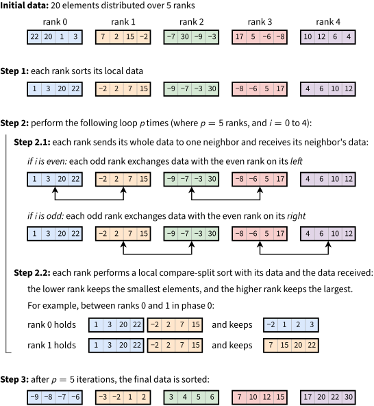
Odd-even sort of 20 elements on \(p = 5\) ranks, colored by rank. Every rank holds 4 elements, so the list is sorted after \(p\) phases. Step 2.2 shows the compare-split of ranks 0 and 1 in phase 0.
The algorithm has the advantage of being very memory-stable, i.e. one can predict the worst-case memory consumption in advance. Moreover, each compute node ends up with the same number of elements it started with, so the initial load balancing across nodes is preserved. However, it is inefficient for a very large network of nodes: on \(p\) ranks, it requires \(p\) phases, and each phase sends all the elements of a node to its neighbor. For a list of \(n\) elements, a rank in the middle of the line thus sends \(p \times n/p = n\) elements, as many as the whole list (20 in the example above).
Distributed Sample Sort
A faster alternative is the distributed sample sort, based on the sample sort, a serial sorting algorithm. Like the bucket sort, it places the elements into buckets of consecutive ranges of values and sorts each bucket. However, it picks the bounds of the buckets from a sample of the data, so that the buckets have about the same size, even when the values are not spread evenly. In the distributed version, each rank is a bucket, and the algorithm is as follows:
- Each compute node sorts its local dataset and collects a few equidistant samples from it;
- Samples are sent to one rank, the root of this gather (rank 0 in the picture below), which sorts them and picks \(p-1\) equidistant samples (the splitters, for \(p\) compute nodes) from the set of received samples;
- The root broadcasts the splitters to the network. The \(p-1\) splitters delimit the range/interval of values to be sent to each of the \(p\) nodes;
- Based on those ranges, the compute nodes perform an all-to-all exchange, a collective scatter-gather in which each element is sent to the appropriate target rank. A first all-to-all of the element counts tells each rank how many elements it receives;
- A final sort of the data in each memory region yields a globally sorted dataset, distributed across the network. As the \(p\) pieces that a rank receives are already sorted, a p-way merge of the pieces, in \(O((n/p) \log p)\) operations, can replace this sort.
Here is an illustrative workflow:
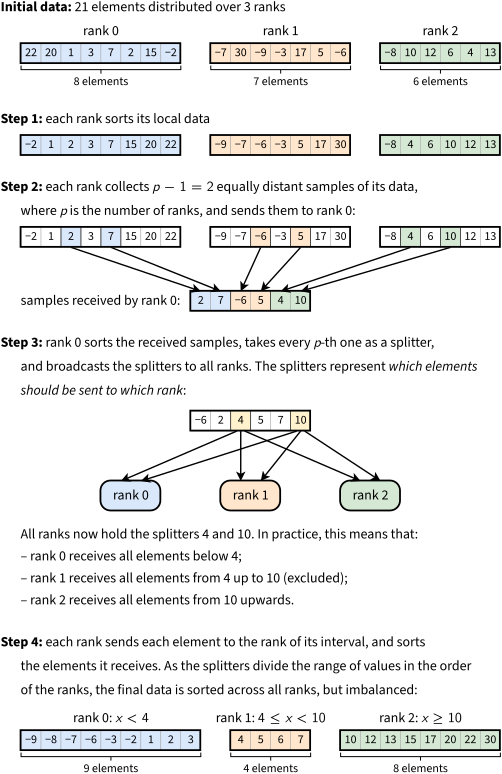
Distributed sample sort of 21 elements on \(p = 3\) ranks, colored by rank. Each rank sends \(p-1 = 2\) samples to rank 0, which sorts them and picks every \(p\)-th one as a splitter (yellow): 4 and 10. The last interval is open: rank 2 receives every element from 10 upwards.
This method is very efficient, as the number of collective calls is constant (a gather, a broadcast and two all-to-alls), regardless of the input size or network size, and each element is sent at most once. Note that the number of calls is constant, but not their size: the root receives \(p-1\) samples from every rank, \(p(p-1)\) in total.
However, it may lead to a highly heterogeneous number of elements across nodes (from 4 to 9 in the example above, for an average of 7), which leads to a computational and memory load imbalance. With regular (equidistant) samples, this imbalance has a bound. In the version of Shi and Schaeffer (1992), called parallel sorting by regular sampling (PSRS), each rank sends \(p\) samples, and no rank receives more than about twice the average, \(2n/p\) elements, when all keys are distinct. If necessary, a network balancing operation may follow the sorting to balance the dataset across the network.
In brief, the distributed sample sort is preferred on large networks, and the odd-even sort on small networks or when each node must keep its number of elements.
The C++ implementation of both algorithms, with MPI, is available in DistributedMemorySorter.cxx and DistributedMemorySorter.h.