Exponential Family of Distributions

The previous post showed that computing the Maximum Likelihood estimator and the Maximum-a-Posteriori on a normally distributed set of parameters becomes much easier once the log-trick is applied. The rationale is that since \(\log\) is a monotonically increasing function, the maximum and minimum of the function to be optimized are attained at the same points as those of the original function inside the \(\log\) operator. Thus, by applying the \(\log\) function, the normal distribution becomes simpler and faster to compute, as a product of exponentials is converted into a sum.

However, this is not a property of the Gaussian distribution only. In fact, most common distributions, including the exponential, log-normal, gamma, chi-squared, beta, Dirichlet, Bernoulli, categorical, Poisson, geometric, inverse Gaussian, von Mises and von Mises-Fisher distributions, can be represented with a similar syntax, making them simple to compute as well. The set of such distributions is called the Exponential Family of Distributions. This post first describes the relationships between common distributions, then defines the exponential family and its properties, derives the parameters of the Gaussian and Bernoulli distributions, and generalizes the maximum likelihood estimator to the whole family.

Detour: relationship between common probability distributions

Probability distributions describe the probabilities of each outcome, with the common property that the probabilities of all outcomes add up to 1. They can also be classified into two subsets: the ones described by a probability mass function, if specified for discrete values, or by a probability density function, if described within some continuous interval. There are dozens (hundreds?) of different distributions, even though only 15 of them are often mentioned and used, and they have some kind of relationship among themselves. The following diagram shows the mass function of each discrete distribution as bars and the density function of each continuous distribution as a curve, with arrows between related distributions:

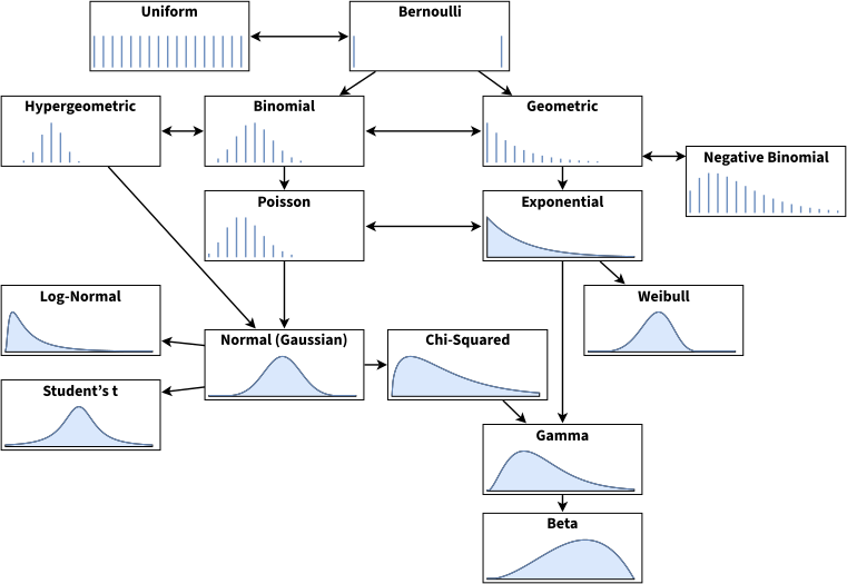
The 15 most common probability distributions and their relationships. Adapted from: Common probability distributions: the data scientist’s crib sheet, S. Owen

A brief summary of their relationships follows. More details are available in the original post by Sean Owen:

• Bernoulli and Uniform: the uniform distribution assigns equal probability to each discrete outcome, e.g. a coin toss or a dice roll; the Bernoulli assigns unequal probabilities \(p\) and \(1-p\) to two discrete outcomes, e.g. an unfair coin toss;
• Binomial and Hypergeometric: the binomial can be seen as the distribution of the sum of outcomes of something that follows a Bernoulli distribution, e.g. if a dice is rolled 30 times, how many times does a six come up? This count follows the binomial distribution, with parameters \(n\), the number of trials, and \(p\), the probability of success (a la Bernoulli). The binomial assumes independent trials, i.e. draws with replacement, while the hypergeometric distribution counts the successes in \(n\) draws without replacement from a finite population that contains a fixed number of successes;
• Poisson and Binomial: like the binomial distribution, the Poisson distribution is a distribution of a count: the number of times some event happened over a fixed interval of time, given a rate for the event to occur. It is parametrized as \(\lambda = np\) (the \(n\) and \(p\) parameters of the binomial, in the limit of a large \(n\) and a small \(p\));
• Geometric and Negative Binomial: while the binomial counts the number of times an event succeeds after a number of trials, the geometric distribution counts how many failed trials occur until the event succeeds. The negative binomial distribution is a simple generalization of the geometric, measuring the number of failures until \(r\) successes have occurred, not only 1 (the table below counts the successes before \(r\) failures instead, which swaps \(p\) and \(1-p\));
• Exponential and Weibull: the exponential distribution is the geometric on a continuous interval, parametrized by \(\lambda\), like the Poisson. While it describes “time until event or failure” at a constant rate, the Weibull distribution models increases or decreases of the rate of failures over time (i.e. models time-to-failure);
• Normal, Log-Normal, Student’s t, and Chi-squared: if one takes a large set of independent values following the same (any) distribution with a finite variance and sums them, that sum approximately follows the normal distribution. This is true regardless of the underlying distribution, and this phenomenon is called the Central Limit Theorem. The log-normal distribution relates to variables whose logarithm is normally distributed. The exponentiation of a normally distributed variable is log-normally distributed. Student’s t-distributions are normal-like distributions with a fatter tail, although they approach the normal distribution as the parameter (the number of degrees of freedom) increases. The chi-squared distribution is the distribution of the sum of squares of independent, standard normally distributed values;
• Gamma and Beta: the gamma distribution is a generalization of the exponential and the chi-squared distributions. Like the exponential distribution, it is used to model waiting times, e.g. the time until the next \(n\) events occur. It appears in machine learning as the conjugate prior to some distributions. The beta distribution is the conjugate prior to the Bernoulli, binomial, negative binomial and geometric distributions.

Exponential Family of distributions

The concept of exponential families dates from 1935–1936, and is credited to E. J. G. Pitman, G. Darmois and B. O. Koopman. The exponential family of distributions is the set of distributions parametrized by \(\theta \in \mathbf{R}^D\) that can be described in the form:

\[p(x \mid \theta) = h(x) \exp \left(\eta(\theta)^T T(x) -A(\theta)\right) \label{eq_main_theta}\]

or in a more extensive notation:

\[p(x \mid \theta) = h(x) \exp\left(\sum_{i=1}^s \eta_i({\boldsymbol \theta}) T_i(x) - A({\boldsymbol \theta}) \right)\]

where \(T(x)\), \(h(x)\), \(\eta(\theta)\), and \(A(\theta)\) are known functions, and \(s\) is the number of components of \(T(x)\). An alternative notation to equation \ref{eq_main_theta} describes \(A\) as a function of \(\eta\), regardless of the transformation from \(\theta\) to \(\eta\). This new expression is called an exponential family in its natural form, and it looks like:

\[p(x \mid \eta) = h(x) \exp \left(\eta^T T(x) -A(\eta)\right) \label{eq_main_eta}\]

The term \(h(x)\) is the base measure, a non-negative function that depends only on \(x\).

The term \(T(x)\) is a sufficient statistic of the distribution. The sufficient statistic is a function of the data that holds all the information the data \(x\) provides with regard to the unknown parameter values:

• The intuitive notion of sufficiency is that \(T(X)\) is sufficient for \(\theta\) if there is no information in \(X\) regarding \(\theta\) beyond that in \(T(X)\). That is, once \(T(X)\) is observed, \(X\) can be thrown away for the purposes of inference with respect to \(\theta\);
• Moreover, this means that the likelihood ratio is the same for any two datasets \(x\) and \(y\) with the same sufficient statistic, i.e. if \(T(x)=T(y)\), then \(\frac{p(x \mid \theta_1)}{p(x \mid \theta_2)} = \frac{p(y \mid \theta_1)}{p(y \mid \theta_2)}\);
• The Pitman–Koopman–Darmois theorem states that, among the families of distributions whose set of possible values does not depend on the parameters, only exponential families have a sufficient statistic whose dimension remains bounded as the number of samples increases.

The term \(\eta\) is the natural parameter, and the set of values of \(\eta\) for which \(A(\eta)\) is finite is called the natural parameter space, which is always convex.

The term \(A(\eta)\) is the log-partition function, because it is the logarithm of a normalization factor that ensures that the distribution \(p(x \mid \theta)\) sums up or integrates to one (without which \(p(x \mid \theta)\) would not be a probability distribution), i.e.:

\[A(\eta) = \log \int_x h(x) \exp (\eta^T T(x)) \, \mathrm{d}x;\]

Another important point is that the mean and variance of \(T(x)\) can be derived by differentiating \(A(\eta)\) and computing its first and second derivatives, respectively:

\[\begin{align*} \frac{dA}{d\eta^T} & = \frac{d}{d\eta^T} \left( \log \int_x h(x) \exp (\eta^T T(x)) \, \mathrm{d}x \right) \\ & = \frac{ \int_x T(x) h(x) \exp (\eta^T T(x)) \, \mathrm{d}x}{\int_x h(x) \exp (\eta^T T(x)) \, \mathrm{d}x} \\ & \qquad \text{(log derivative rule: } \frac{d}{dx} \log f(x) = \frac{f'(x)}{f(x)} \text{)} \\ & = \int_x T(x) h(x) \exp(\eta^TT(x) - A(\eta)) \, \mathrm{d}x \\ & \qquad \text{(definition of } p(x \mid \eta) \text{, and } \frac{e^a}{e^b} = e^{a-b} \text{)} \\ & = \mathbf{E}[T(X)] \\ & \qquad \text{(def. expected value: } \mathbf{E}[X] = \int_x x \, f(x) dx \text{, for density func. } f(x) \text{)} \\ \end{align*}\]

i.e. the first derivative of \(A(\eta)\) is equal to the mean of the sufficient statistic. Now consider the second derivative:

\[\begin{align*} \frac{d^2A}{d\eta\,d\eta^T} & = \int_x h(x) T(x) \left( T(x) -\frac{d}{d\eta^T}A(\eta)\right)^T \, \exp\left(\eta^TT(x) - A(\eta)\right) \, dx \\ & = \int_x h(x) T(x) \left( T(x) - \mathbf{E}[T(X)] \right)^T \, \exp\left(\eta^TT(x) - A(\eta)\right) \, dx & (\frac{dA}{d\eta^T} = \mathbf{E}[T(X)])\\ & = \mathbf{E}[T(X)T(X)^T] -\mathbf{E}[T(X)] \, \mathbf{E}[T(X)]^T & (\mathbf{E}[X] = \int_x x \, f(x) dx)\\ & = \mathbf{Var}[T(X)] & (Var(X)=E[X^2]-E[X]^2)\\ \end{align*}\]

and, as expected, the second derivative is equal to the variance of \(T(X)\).

One requirement of exponential family distributions is that the density must factorize (i.e. must be separable into products, each involving only one type of variable, \(x\) or \(\theta\)), as either the power or the base of an exponentiation operation. I.e. the factors must be one of the following:

\[f(x), g(\theta), c^{f(x)}, c^{g(\theta)}, {[f(x)]}^c, {[g(\theta)]}^c, {[f(x)]}^{g(\theta)}, {[g(\theta)]}^{f(x)}, {[f(x)]}^{h(x)g(\theta)}, \text{ or } {[g(\theta)]}^{h(x)j(\theta)}\]

where \(f\) and \(h\) are arbitrary functions of \(x\), \(g\) and \(j\) are arbitrary functions of \(\theta\); and \(c\) is an arbitrary constant expression.

Another important point is that the product of two exponential-family distributions is also part of the exponential family, but unnormalized:

\[\left[ h(x) \exp \left(\eta_1^T T(x) -A(\eta_1)\right) \right] * \left[ h(x) \exp \left(\eta_2^T T(x) -A(\eta_2)\right) \right] = \widetilde{h}(x) \exp \left(\left(\eta_1+\eta_2\right)^T T(x) -\widetilde{A}(\eta_1, \eta_2)\right)\]

where \(\widetilde{h}(x) = h(x)^2\) and \(\widetilde{A}(\eta_1, \eta_2) = A(\eta_1) + A(\eta_2)\).

Finally, exponential family distributions have conjugate priors, i.e. priors for which the posterior distribution is in the same family as the prior. With such priors, the posterior predictive distribution always has a closed-form solution (provided that the normalizing factor can also be stated in closed form). Both are important properties for Bayesian statistics.

Example: Univariate Gaussian distribution

The univariate Gaussian distribution is defined for an input \(x\) as:

\[p(x \mid \mu, \sigma^2 ) = \frac{1}{ \sqrt{2 \pi \sigma^2} } \,\, \exp \left( - \frac{(x - \mu)^2}{2 \sigma^2} \right)\]

for a distribution with mean \(\mu\) and standard deviation \(\sigma\). By moving the terms around, the density can be written as:

\[\begin{align*} %% source: http://www.cs.columbia.edu/~jebara/4771/tutorials/lecture12.pdf p(x \mid \mu, \sigma ) & = \frac{1}{ \sqrt{2 \pi \sigma^2} } \,\, \exp \left( - \frac{(x - \mu)^2}{2 \sigma^2} \right) \\ & = \frac{1}{ \sqrt{2 \pi } } \,\, \exp \left( - \log \sigma - \frac{x^2}{2 \sigma^2} + \frac{\mu x}{\sigma^2} - \frac{\mu^2}{2 \sigma^2} \right) \\ & = \frac{1}{ \sqrt{2 \pi } } \,\, \exp \left( \eta(\theta)^TT(x) - \log \sigma - \frac{\mu^2}{2\sigma^2} \right) \\ & = h(x) \,\, \exp \left( \eta(\theta)^TT(x) - A(\theta) \right) \\ \end{align*}\]

where:

• \(h(x) = \frac{1}{ \sqrt{2 \pi}}\),
• \(T = { x \choose x^2 }\),
• \(\eta(\theta) = { \mu/(\sigma^2) \choose -1/(2\sigma^2) }\),
• \(A(\eta) = \frac{\mu^2}{2\sigma^2} + \log \sigma = - \frac{ \eta^2_1}{4 \eta_2} - \frac{1}{2} \log(-2\eta_2)\).

The first and second derivatives of \(A(\eta)\) are now used to compute the mean and the variance of the sufficient statistic \(T(x)\):

\[\begin{align*} %% source: https://people.eecs.berkeley.edu/~jordan/courses/260-spring10/other-readings/chapter8.pdf \frac{dA}{d\eta_1} & = \frac{d}{d\eta_1} \left( - \frac{ \eta^2_1}{4 \eta_2} - \frac{1}{2} \log(-2\eta_2) \right) \\ & = -\frac{\eta_1}{2\eta_2} \\ & = \frac{\mu / \sigma^2}{1/\sigma^2} \\ & = \mu \\ \end{align*}\]

which is the mean of \(x\), the first component of the sufficient statistic. Taking the second derivative yields:

\[%% source: https://people.eecs.berkeley.edu/~jordan/courses/260-spring10/other-readings/chapter8.pdf \frac{d^2A}{d\eta_1^2} = - \frac{1}{2\eta_2} = \sigma^2\]

which is the variance of the normal distribution, by definition.

Example: Bernoulli distribution

Similarly, the exponential family parameters of the Bernoulli distribution are computed as follows:

\[%% source: http://www.cs.columbia.edu/~jebara/4771/tutorials/lecture12.pdf \begin{align*} p(x \mid \alpha) & = \alpha^x (1-\alpha)^{1-x} \hspace{0.5cm}, x \in \{0,1\} \\ & = \exp \left( \log (\alpha^x (1-\alpha)^{1-x}) \right) \\ & = \exp \left( x \log \alpha + (1-x) \log (1-\alpha) \right) \\ & = \exp \left( x \log \frac{\alpha}{1-\alpha} + \log (1-\alpha) \right) \\ & = \exp \left( x \eta - \log (1+e^\eta) \right) \\ \end{align*}\]

where:

• \(h(x) = 1\),
• \(T(x) = x\),
• \(\eta = \log \frac{\alpha}{1-\alpha}\),
• \(A(\eta) = \log ( 1+e^\eta)\).

The mean of \(T(x)\) is now computed as:

\[\begin{align*} \frac{d A}{d \eta} = \frac{e^\eta}{1+e^\eta} = \frac{1}{1 + e^{-\eta}} = \mu \\ \end{align*}\]

which is the mean \(\mu = \alpha\) of a Bernoulli variable. Taking a second derivative yields:

\[%% source: https://people.eecs.berkeley.edu/~jordan/courses/260-spring10/other-readings/chapter8.pdf \frac{d^2A}{d\eta^2} = \frac{d \mu}{d \eta} = \mu (1-\mu)\]

which is the variance of a Bernoulli variable.

Parameters for common distributions

The following table provides a summary of the most common distributions in the exponential family and their exponential-family parameters. A more exhaustive list is available in the Wikipedia entry for Exponential Family. Note that the rows of the Bernoulli distribution and of the normal distribution with unknown variance hold the parameters derived in the examples above, with \(p\) in place of \(\alpha\).

Distribution	Probability Density/Mass Function	Natural parameter(s) \(\boldsymbol\eta\)	Inverse parameter mapping	Base measure \(h(x)\)	Sufficient statistic \(T(x)\)	Log-partition \(A(\boldsymbol\eta)\)	Log-partition \(A(\boldsymbol\theta)\)
Bernoulli distribution	\(f(x ; p) = p^x (1-p)^{1-x}\)	\(\log\frac{p}{1-p}\) (logit function)	\(\frac{1}{1+e^{-\eta}} = \frac{e^\eta}{1+e^{\eta}}\) (logistic function)	\(1\)	\(x\)	\(\log (1+e^{\eta})\)	\(-\log (1-p)\)
binomial distribution with known number of trials n	\(f(x; n,p) = \binom{n}{x}p^x(1-p)^{n-x} \)	\(\log\frac{p}{1-p}\)	\(\frac{1}{1+e^{-\eta}} = \frac{e^\eta}{1+e^{\eta}}\)	\({n \choose x}\)	\(x\)	\(n \log (1+e^{\eta})\)	\(-n \log (1-p)\)
Poisson distribution	\( f(x; \lambda)=\frac{\lambda^x e^{-\lambda}}{x!}\)	\(\log\lambda\)	\(e^\eta\)	\(\frac{1}{x!}\)	\(x\)	\(e^{\eta}\)	\(\lambda\)
negative binomial distribution with known number of failures r	\( f(x; r, p) = \binom{x+r-1}{x} p^x(1-p)^r \)	\(\log p\)	\(e^\eta\)	\({x+r-1 \choose x}\)	\(x\)	\(-r \log (1-e^{\eta})\)	\(-r \log (1-p)\)
exponential distribution	\( f(x;\lambda) = \begin{cases} \lambda e^{-\lambda x} & x \ge 0, \\ 0 & x < 0. \end{cases} \)	\(-\lambda\)	\(-\eta\)	\(1\)	\(x\)	\(-\log(-\eta)\)	\(-\log\lambda\)
Pareto distribution with known minimum value \( x_m \)	\( f(x;\alpha) = \begin{cases} \frac{\alpha x_\mathrm{m}^\alpha}{x^{\alpha+1}} & x\ge x_\mathrm{m}, \\ 0 & x < x_\mathrm{m}. \end{cases} \)	\(-\alpha-1\)	\(-1-\eta\)	\(1\)	\(\log x\)	\(-\log (-1-\eta) + (1+\eta) \log x_{\mathrm m}\)	\(-\log \alpha - \alpha \log x_{\mathrm m}\)
Laplace distribution with known mean μ	\( f(x ; \mu,b) = \frac{1}{2b} \exp \left( -\frac{|x-\mu|}{b} \right) \\ = \frac{1}{2b} \left\{\begin{matrix} \exp \left( -\frac{\mu-x}{b} \right) & \text{if }x < \mu \\[8pt] \exp \left( -\frac{x-\mu}{b} \right) & \text{if }x \geq \mu \end{matrix}\right. \)	\(-\frac{1}{b}\)	\(-\frac{1}{\eta}\)	\(1\)	\(|x-\mu|\)	\(\log\left(-\frac{2}{\eta}\right)\)	\(\log 2b\)
normal distribution known variance	\( f(x; \mu, \sigma^2) = \frac{1}{\sigma \sqrt{2\pi} } e^{-\frac{1}{2}\left(\frac{x-\mu}{\sigma}\right)^2} \)	\(\mu/\sigma\)	\(\sigma\eta\)	\(\frac{e^{-\frac{x^2}{2\sigma^2}}}{\sqrt{2\pi}\sigma}\)	\(\frac{x}{\sigma}\)	\(\frac{\eta^2}{2}\)	\(\frac{\mu^2}{2\sigma^2}\)
normal distribution	\( f(x; \mu, \sigma^2) = \frac{1}{\sigma \sqrt{2\pi} } e^{-\frac{1}{2}\left(\frac{x-\mu}{\sigma}\right)^2} \)	\(\begin{bmatrix} \dfrac{\mu}{\sigma^2} \\[10pt] -\dfrac{1}{2\sigma^2} \end{bmatrix}\)	\(\begin{bmatrix} -\dfrac{\eta_1}{2\eta_2} \\[15pt] -\dfrac{1}{2\eta_2} \end{bmatrix}\)	\(\frac{1}{\sqrt{2\pi}}\)	\(\begin{bmatrix} x \\ x^2 \end{bmatrix}\)	\(-\frac{\eta_1^2}{4\eta_2} - \frac12\log(-2\eta_2)\)	\(\frac{\mu^2}{2\sigma^2} + \log \sigma\)
lognormal distribution	\( \ln(X) \sim \mathcal N(\mu,\sigma^2) \)	\(\begin{bmatrix} \dfrac{\mu}{\sigma^2} \\[10pt] -\dfrac{1}{2\sigma^2} \end{bmatrix}\)	\(\begin{bmatrix} -\dfrac{\eta_1}{2\eta_2} \\[15pt] -\dfrac{1}{2\eta_2} \end{bmatrix}\)	\(\frac{1}{\sqrt{2\pi}x}\)	\(\begin{bmatrix} \log x \\ (\log x)^2 \end{bmatrix}\)	\(-\frac{\eta_1^2}{4\eta_2} - \frac12\log(-2\eta_2)\)	\(\frac{\mu^2}{2\sigma^2} + \log \sigma\)
gamma distribution shape \(\alpha\), rate \(\beta\)	\( f(x;\alpha,\beta) = \frac{ \beta^\alpha x^{\alpha-1} e^{-\beta x}}{\Gamma(\alpha)} \\ (\text{ for } x > 0 \quad \alpha, \beta > 0) \)	\(\begin{bmatrix} \alpha-1 \\ -\beta \end{bmatrix}\)	\(\begin{bmatrix} \eta_1+1 \\ -\eta_2 \end{bmatrix}\)	\(1\)	\(\begin{bmatrix} \log x \\ x \end{bmatrix}\)	\(\log \Gamma(\eta_1+1)-(\eta_1+1)\log(-\eta_2)\)	\(\log \Gamma(\alpha)-\alpha\log\beta\)
gamma distribution shape \(k\), scale \(\theta\)	\( f(x;k,\theta) = \frac{x^{k-1}e^{-\frac{x}{\theta}}}{\theta^k\Gamma(k)} \\ (\text{ for } x > 0 \text{ and } k, \theta > 0) \)	\(\begin{bmatrix} k-1 \\[5pt] -\dfrac{1}{\theta} \end{bmatrix}\)	\(\begin{bmatrix} \eta_1+1 \\[5pt] -\dfrac{1}{\eta_2} \end{bmatrix}\)	\(1\)	\(\begin{bmatrix} \log x \\ x \end{bmatrix}\)	\(\log \Gamma(\eta_1+1)-(\eta_1+1)\log(-\eta_2)\)	\(\log \Gamma(k)+k\log\theta\)
beta distribution	\( f(x;\alpha,\beta) = \frac{1}{B(\alpha,\beta)} x^{\alpha-1}(1-x)^{\beta-1} \)	\(\begin{bmatrix} \alpha \\ \beta \end{bmatrix}\)	\(\begin{bmatrix} \eta_1 \\ \eta_2 \end{bmatrix}\)	\(\frac{1}{x(1-x)}\)	\(\begin{bmatrix} \log x \\ \log (1-x) \end{bmatrix}\)	\(\log \Gamma(\eta_1) + \log \Gamma(\eta_2)\\- \log \Gamma(\eta_1+\eta_2)\)	\(\log \Gamma(\alpha) + \log \Gamma(\beta)\\- \log \Gamma(\alpha+\beta)\)
multivariate normal distribution	\( f(x; \mu, \Sigma) = (2\pi)^{-\frac{k}{2}}\det(\Sigma)^{-\frac{1}{2}} \\ \,\, \exp \left( -\frac{1}{2}(x - \mu)^T\Sigma^{-1}(x - \mu) \right)\)	\(\begin{bmatrix} \boldsymbol\Sigma^{-1}\boldsymbol\mu \\[5pt] -\frac12\boldsymbol\Sigma^{-1} \end{bmatrix}\)	\(\begin{bmatrix} -\frac12\boldsymbol\eta_2^{-1}\boldsymbol\eta_1 \\[5pt] -\frac12\boldsymbol\eta_2^{-1} \end{bmatrix}\)	\((2\pi)^{-\frac{k}{2}}\)	\(\begin{bmatrix} \mathbf{x} \\[5pt] \mathbf{x}\mathbf{x}^\mathrm{T} \end{bmatrix}\)	\(-\frac{1}{4}\boldsymbol\eta_1^{\rm T}\boldsymbol\eta_2^{-1}\boldsymbol\eta_1 - \frac12\log\left|-2\boldsymbol\eta_2\right|\)	\(\frac12\boldsymbol\mu^{\rm T}\boldsymbol\Sigma^{-1}\boldsymbol\mu + \frac12 \log |\boldsymbol\Sigma|\)
multinomial distribution with known number of trials n	\( f(x_1,\ldots,x_k;n,p_1,\ldots,p_k) = \\ \frac{n!}{x_1!\cdots x_k!} p_1^{x_1} \cdots p_k^{x_k} \\ \text{(where } \sum_{i=1}^k p_i = 1 \text{)} \)	\(\begin{bmatrix} \log p_1 \\ \vdots \\ \log p_k \end{bmatrix}\)	\(\begin{bmatrix} e^{\eta_1} \\ \vdots \\ e^{\eta_k} \end{bmatrix}\) where \(\textstyle\sum_{i=1}^k e^{\eta_i}=1\)	\(\frac{n!}{\prod_{i=1}^{k} x_i!}\)	\(\begin{bmatrix} x_1 \\ \vdots \\ x_k \end{bmatrix}\)	\(0\)	\(0\)

Maximum Likelihood

This post has shown that the Gaussian, alongside plenty of other distributions, belongs to the Exponential Family of Distributions. This section shows that the Maximum Likelihood Estimator (MLE) can be generalized across all distributions in the Exponential Family.

As in the Gaussian case, the computation of the MLE starts by applying the log-trick to the general expression of the exponential family, which gives the following log-likelihood for the complete dataset \(X=(x_1, x_2, ..., x_N)\) of \(N\) independent samples:

\[%% source: http://www.cs.columbia.edu/~jebara/4771/tutorials/lecture12.pdf \begin{align*} lik(\eta \mid X) &= \log p(X \mid \eta) \\ & = \log \left( \prod_{i=1}^N h(x_i) \exp \left(\eta^T T(x_i) -A(\eta) \right) \right) \\ & = \log \left( \prod_{i=1}^N h(x_i) \right) + \eta^T \left( \sum_{i=1}^N T(x_i) \right) - NA(\eta) \\ %\log p(x \mid \eta) & = \sum_{i=1}^N \log p(x_i \mid \theta) \\ % & = \sum_{i=1}^M \log \left( h(x_i) \exp \left(\eta(\theta)^T T(x_i) -A(\theta) \right) \right) \\ % & = \sum_{i=1}^N \left( \log h(x_i) + \eta(\theta)^T T(x_i) - A(\theta) \right) \\ % & = \sum_{i=1}^N \left( \log h(x_i) + \eta(\theta)^T T(x_i) \right) - NA(\theta) \\ \end{align*}\]

The derivative with respect to \(\eta\) is then computed and set to zero, which gives the maximum likelihood estimate of the mean parameter \(\boldsymbol{\mu} = \mathbf{E}[T(X)]\):

\[%% source: http://www.cs.columbia.edu/~jebara/4771/tutorials/lecture12.pdf \begin{align*} & \frac{d}{d \eta} lik(\eta \mid X) = 0 \\ \Leftrightarrow & \sum_{i=1}^N T(x_i) - N \nabla_\eta A (\eta) =0 \\ \Leftrightarrow & \nabla_\eta A (\eta) = \frac{1}{N} \sum_{i=1}^N T(x_i)\\ \Leftrightarrow & \boldsymbol{\mu}_{MLE} = \frac{1}{N} \sum_{i=1}^N T(x_i) \\ & \qquad \text{(from above: } \frac{dA(\eta)}{d \eta} = \mathbf{E}[T(X)] \text{ and } \mathbf{E}[T(X)] = \boldsymbol{\mu} \text{)} \\ \end{align*}\]

Not surprisingly, the result relates to the data only via the sufficient statistic \(\sum_{i=1}^N T(x_i)\), giving a meaning to the notion of sufficiency: to estimate parameters, only the sufficient statistic is retained. For distributions in which \(T(x) = x\), which include the Bernoulli, Poisson and multinomial distributions, it shows that the sample mean is the maximum likelihood estimate of the mean. For the univariate Gaussian distribution, the sample mean is the maximum likelihood estimate of the mean and the sample variance (with the factor \(1/N\), not \(1/(N-1)\)) is the maximum likelihood estimate of the variance.

To find more about the topic, the moments and the maximum likelihood estimate of this post are derived in more detail in chapter 8 of the draft book An Introduction to Probabilistic Graphical Models by Michael I. Jordan, The exponential family: Basics. The chapter also proves that the natural parameter space and the log-partition function are convex, and shows that maximizing the likelihood is equivalent to minimizing the Kullback–Leibler divergence to the empirical distribution of the data.