The Leaky Integrate-and-Fire Neuron and the Brunel Network
The Leaky Integrate-and-Fire (LIF) neuron model describes a neuron by a single variable, its membrane potential: it integrates the input current, leaks back to rest, and makes the neuron fire a spike when it reaches a threshold.
The LIF neuron model
The LIF model, first described in 1907 by Louis Lapicque, simplifies the structure of a neuron to a single leaky compartment (point neuron model), with a membrane described by an RC circuit. The membrane separates electric charges as a capacitor does, and its ion channels let a current leak through it as a resistor does. The circuit is the following:
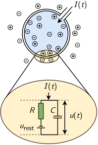
A neuron receives an input current \(I(t)\). Its membrane acts as a capacitor \(C\) in parallel with a resistor \(R\), in series with a battery of potential \(u_{\text{rest}}\). Adapted from: Neuronal Dynamics, Fig. 1.6
The main formulation of its electrical activity is given by the current equation, with the following terms:
- The current in the capacitor \(C\) is given by \(I_C = \frac{dQ}{dt} = \frac{d(CV)}{dt} = C \frac{dV}{dt}\), for charge \(Q\) and capacitance \(C\);
- The current in the resistance \(R\) is given by Ohm’s law as \(I_R = V/R\), for the membrane potential \(V\) (relative to the resting potential \(u_{\text{rest}}\)) and resistance \(R\).
The law of conservation of electric charge states that the total charge of an isolated system remains constant. Thus, the currents entering a node of the circuit sum to the currents leaving it (Kirchhoff’s current law), i.e. the input current is \(I = I_C + I_R\). Equivalently:
\[C \frac{dV}{dt}(t) = -\frac{V(t)}{R} + I(t)\]It is common to multiply all terms by \(R\) to expose the time constant \(\tau = R C\). This is a very important metric in the analysis of the behavior of models, as it tells how fast the dynamics of the neuron are. The formulation then becomes:
\[\tau \frac{dV}{dt}(t) = -V(t) + RI(t) \label{equation_diff}\]The external currents (such as synaptic activity) are added to \(I(t)\). In practice, the network contribution \(R I_i(t)\) to a neuron \(i\) is the sum of all currents delivered to it by any neuron \(j\) over time, and is described as:
\[R I_i(t) = \tau \sum_{j} J_{ij} \sum_{t^\prime} \delta (t-t^\prime _{j} -D) \label{equation_current}\]where \(J_{ij}\) is the postsynaptic potential (PSP) amplitude of the synapse from neuron \(j\) to neuron \(i\), \(\delta (t)\) the Dirac delta function, \(t^\prime _{j}\) the spiking times \(t^\prime\) of the presynaptic neuron \(j\), and \(D\) the synaptic (or transmission) delay. For simplicity, the index \(i\) is dropped from here on, and \(V(t)\) is represented as \(V_t\).
The neuron’s potential is considered to rise steeply when there is an input current (by \(J_{ij}\) at each input spike), thus discarding the exponential charging of the capacitor. On the other hand, the discharge follows an exponential decay with the time constant \(\tau\).
To simulate the action potential (or spike) of biological neurons, the model assumes that each neuron has a certain fixed firing threshold. When the potential reaches the firing threshold, the neuron spikes (or fires), and its potential immediately drops to a reset potential. Axonal branches of neurons are simulated by a synaptic delay that regulates the time a spike signal takes to reach the connected postsynaptic neurons. This propagation of spike and current, which dictates the synaptic delay, is illustrated in the following picture:
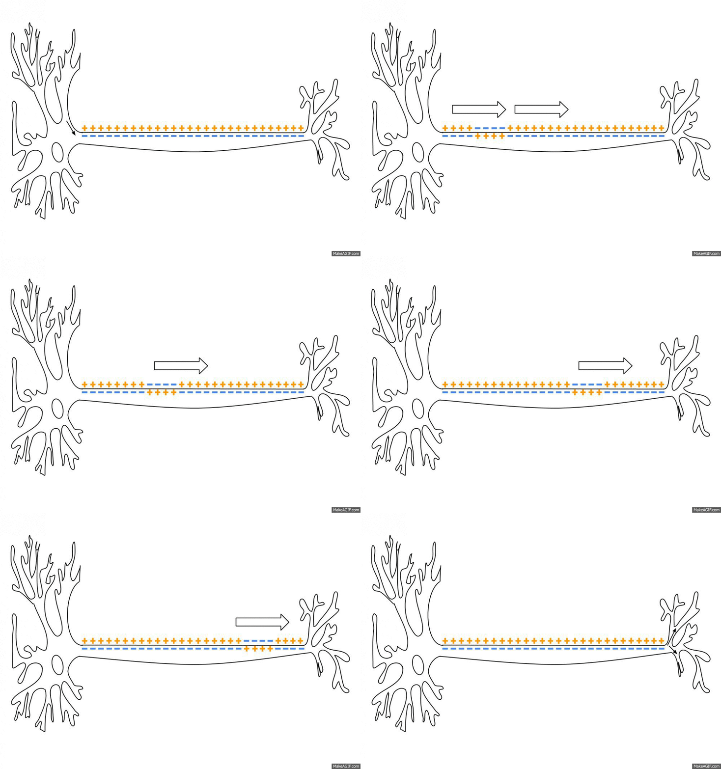
An action potential travelling along an axon, in the direction of the arrows. The membrane is positive outside and negative inside, except at the action potential, where the polarity is reversed. Source: Action Potential.gif, Wikimedia Commons

Afterwards, for a given refractory period \(\tau_{\text{rp}}\), the neuron potential stays constant at the reset value, to simulate the refraction of biological neurons. Therefore, a neuron fires at most \(1/\tau_{\text{rp}}\) times per second, 500 times for the 2 ms of the network of this post.
Integration methods
Exact integration
The jumps and the exponential decay described above are the exact solution of equation \ref{equation_diff}. Between two input spikes, the input current is zero, and the equation reduces to \(\tau \frac{dV}{dt} = -V\). Its solution is an exponential decay towards the resting potential:
\[V(t) = V(t_0) \exp\left(-\frac{t - t_0}{\tau}\right)\]where \(t_0\) is the time of the last input spike. At an input spike, the potential jumps by \(J_{ij}\). Indeed, when equation \ref{equation_diff} is integrated over an infinitely short interval around the arrival of the spike, the leak term vanishes, and the delta current of equation \ref{equation_current} gives \(\tau \Delta V = \tau J_{ij}\).
In practice, each input raises the potential only a little, and the leak pulls it back to rest. Therefore, the neuron fires only when many inputs arrive within a short time, before the leak brings its potential back to rest.
Two different stepping methods are derived from the analytical solution of the first-order ODE, both based on a two-step algorithm:
- Calculate the decay from the previous step: \(V_t \leftarrow V_{t- \Delta t} \exp(\frac{-\Delta t}{\tau})\)
- Add the voltage change due to the network current \(RI\) between \(t-\Delta t\) and \(t\): \(V_t \leftarrow V_t + RI_{(t-\Delta t, t]} / \tau\), where \(RI_{(t-\Delta t, t]}\) is the integral of \(RI\) over that interval, i.e. \(\tau\) times the sum of the amplitudes \(J_{ij}\) of the spikes that arrive in it.
Neurons can be advanced with fixed-step or variable-step integration:
- Fixed step integration assumes the time step \(\Delta t\) to be constant throughout the execution.
- Variable step methods advance the neuron with the smallest \(t\) in the network, with a \(\Delta t\) computed as the minimum of the following two values:
- the time difference to the next incoming spike, so that each spike is added at its exact time;
- \(t^\star + D - t\), where \(t^\star\) is the time of the neuron with the second smallest \(t\) and \(D\) is the synaptic delay, i.e. the largest step that can be taken from the neuron at \(t\) without missing a spike from the neuron at time \(t^\star\) (if it spikes).
Euler methods
The fixed and variable step integrations can also be computed numerically, instead of using the analytical solution. This is common practice for efficiency purposes, as the required exponential and division operations are computationally costly when \(\Delta t\) changes at every step. The solution is not exact, but it approximates the exact solution well enough when the timestep \(\Delta t\) is small enough. As a simple example, two approximate fixed-step Euler methods can be used:
- Explicit Forward Euler:
- Implicit Backward Euler:
with \(\frac{dV_{t}}{dt}\) and \(RI_{(t-\Delta t, t]}\) computed from equations \ref{equation_diff} and \ref{equation_current}, respectively. Note that \(RI_{(t-\Delta t, t]}\) is divided by \(\Delta t\) so that it is expressed per time unit instead of per timestep.
Comparison of the methods
With a fixed step, however, the three methods have the same cost, as the factor \(\exp(\frac{-\Delta t}{\tau})\) of the analytical solution is a constant, computed only once. They differ in the factor that multiplies the potential of the previous step. Rearranged, the three updates are:
\[\begin{align*} \text{exact:} \quad & V_t = \exp(\frac{-\Delta t}{\tau}) \, V_{t-\Delta t} + RI_{(t-\Delta t, t]} / \tau \\ \text{explicit Euler:} \quad & V_t = (1 - \frac{\Delta t}{\tau}) \, V_{t-\Delta t} + RI_{(t-\Delta t, t]} / \tau \\ \text{implicit Euler:} \quad & V_t = \frac{\tau}{\tau + \Delta t} \, (V_{t-\Delta t} + RI_{(t-\Delta t, t]} / \tau) \end{align*}\]For a step much smaller than \(\tau\), as in the Brunel network below, the three factors are almost equal, and so are the three methods. However, explicit Euler is stable only for \(\Delta t < 2 \tau\), while implicit Euler is stable for any \(\Delta t\).
The variable step method is an event-driven algorithm: it is the most accurate, as each spike is added at its exact time, but it advances one neuron at a time. The fixed step methods are clock-driven (or time-driven): they advance all neurons together at every step, but align the spike times to the time grid. In practice, the fixed step suits large networks, as all neurons run the same operations at every step, while the variable step suits models where the exact timing of spikes matters.
For the sake of comparison, the picture below illustrates the potential over time of a given neuron in a network, for the aforementioned methods. The simulation runs for 100 ms on a Brunel network of 10,000 neurons, with the parameters of the next section. Results are given for the implicit and explicit Euler methods with \(\Delta t = 0.1\) ms, and for the analytical solution with fixed (\(\Delta t = 0.1\) ms) and variable time steps:
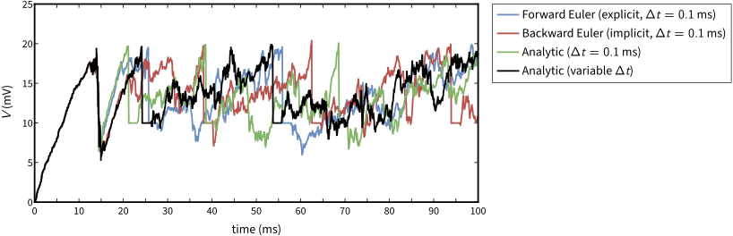
Note the vertical straight lines, which refer to the voltage reset after a spike, and the horizontal straight lines, which refer to the refractory period after firing. During the first 12 ms, the four curves overlap, as the factors of the methods differ by about 0.001% per step. They diverge once the first spikes of the network reach the neuron, as a small difference in a spike time changes the input of all postsynaptic neurons.
The Brunel network
A neuron without any stimulus (either electric current injection or synaptic currents) always remains at rest.
One of the most common models of network activity is the Brunel network model (Dynamics of Sparsely Connected Networks of Excitatory and Inhibitory Spiking Neurons, Brunel, Journal of Computational Neuroscience, 2000, pdf). It is highly relevant, as it comes with a theory that predicts its dynamics. A mean-field analysis replaces the input that each neuron receives from the network by its average and its fluctuations. A Fokker-Planck equation for the distribution of the membrane potentials then gives the firing rates and the states of the network.
The model proposes a network of 10,000 simulated LIF neurons (80% excitatory, 20% inhibitory; the paper simulates 12,500). Its connections are sparse and random: each neuron receives inputs from 10% of the excitatory and 10% of the inhibitory neurons. External stimuli come from excitatory neurons outside the network, which connect to both the excitatory and the inhibitory neurons. Excitatory means that the PSP is positive; the converse holds for inhibitory neurons. The external neurons are not simulated, so their spiking is generated by a Poisson random generator (PG). The diagram is the following:
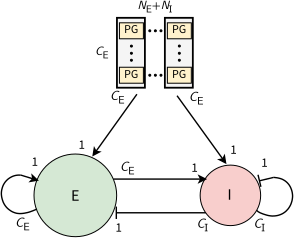
The Brunel network: \(N_E\) excitatory neurons (E) and \(N_I\) inhibitory neurons (I). Each neuron receives \(C_E\) connections from excitatory neurons, \(C_I\) from inhibitory neurons, and \(C_E\) from Poisson generators (PG). Arrows are excitatory connections, and flat bars inhibitory ones. Adapted from: NEST by Example, Fig. 2
The tricky part here is to define the parameters of the network in terms of connectivity, synaptic weights, firing threshold, etc. The original paper describes them in detail, but for simplicity, they are summarized in the tables below:
| Network Parameters | |
|---|---|
| Parameter | Value |
| Number of excitatory neurons \(N_E\) | 8000 |
| Number of inhibitory neurons \(N_I\) | 2000 |
| Excitatory synapses per neuron \(C_E\) | 800 |
| Inhibitory synapses per neuron \(C_I\) | 200 |
| Neuron Parameters | |
|---|---|
| Parameter | Value |
| Membrane time constant \(\tau\) | 20 ms |
| Refractory period \(\tau_{\text{rp}}\) | 2 ms |
| Firing threshold \(V_{\text{th}}\) | 20 mV |
| Membrane capacitance \(C\) | 1 pF |
| Resting potential \(u_{\text{rest}}\) | 0 mV |
| Reset potential \(V_{\text{reset}}\) | 10 mV |
| Excitatory PSP amplitude \(J_E\) | 0.1 mV |
| Inhibitory PSP amplitude \(J_I\) | -0.5 mV |
| Synaptic delay \(D\) | 1.5 ms |
| Background rate \(\eta\) | 2.0 |
source: Marc-Oliver Gewaltig, ResearchGate
Network states
The stimuli parameters can now be adjusted to regulate network activity. The background rate \(\eta\) sets the rate \(\nu_{\text{ext}}\) of each Poisson generator. It is given in units of the threshold rate \(\nu_{\text{thr}}\), at which the external input alone brings the mean potential of a neuron to its threshold:
\[\nu_{\text{ext}} = \eta \, \nu_{\text{thr}}, \quad \text{with} \quad \nu_{\text{thr}} = \frac{V_{\text{th}}}{J_E C_E \tau}\]With \(\eta = 2\), the external input alone would bring the mean potential to \(\eta V_{\text{th}}\), twice the threshold. Starting from rest, the potentials of the neurons then reach the threshold at about the same time, and the network fires a first wave of spikes (the first bars of the AI plot below).
The relative strength \(g\) of the inhibitory synapses sets \(J_I = -g J_E\) (the table above has \(J_I = -0.5\) mV, i.e. \(g = 5\)), and decides whether excitation or inhibition dominates. When the neurons of the network fire at a rate \(\nu\), the mean input that a neuron receives from the network is computed as:
\[\mu_{\text{rec}} = \tau \nu (C_E J_E + C_I J_I) = C_E J_E \tau \nu \left(1 - g \frac{C_I}{C_E}\right)\]Each neuron receives four times as many excitatory inputs as inhibitory ones (\(C_I / C_E = 1/4\)), so this input is zero at \(g = 4\), the balance of excitation and inhibition. In Brunel’s words, the line \(g = 4\) “is where feedback excitation exactly balances inhibition”. The network is excitation-dominated for \(g < 4\), and inhibition-dominated for \(g > 4\). The plot of the previous section shows it: at \(g = 5\), the first wave of spikes reaches the neuron after the synaptic delay, at around 14.5 ms, and its potential falls by 10 to 14 mV instead of rising.
Depending on \(g\) and \(\eta\), Brunel describes four states of the network. They are named after the global activity of the network, synchronous when it oscillates and asynchronous when it is stationary, and after the firing of each neuron, regular or irregular. In the synchronous regular (SR) state, excitation dominates (\(g = 3\)), and the neurons fire regularly at high rates, almost all together. Inhibition dominates in the three other states, where each neuron fires irregularly. The global activity is stationary in the asynchronous irregular (AI) state, and oscillates fast or slowly in the synchronous irregular (SI) states, SI fast and SI slow.
The following table gives the values of \(g\) and \(\eta\) of each state in the simulations of the paper (Fig. 8 in the paper). For the three inhibition-dominated states, it also gives the average firing rates and global oscillation frequencies of the simulations and of the theory (Table 1 in the paper):
| State | \(g\) | \(\eta\) | Firing rate | Global frequency | ||
|---|---|---|---|---|---|---|
| Simulation | Theory | Simulation | Theory | |||
| SR | 3 | 2 | not compared in the paper | |||
| SI, fast | 6 | 4 | 60.7 Hz | 55.8 Hz | 180 Hz | 190 Hz |
| AI | 5 | 2 | 37.7 Hz | 38.0 Hz | — | — |
| SI, slow | 4.5 | 0.9 | 5.5 Hz | 6.5 Hz | 22 Hz | 29 Hz |
source: Brunel 2000
Notice how close the simulated network is to the theoretical predictions: within 1% for the firing rate of the AI state, and within 25% for the firing rates and global frequencies of the SI states. For that reason, although it is a simple approximation, the Brunel network is a powerful tool for studying network dynamics. The model is particularly useful in very long simulations of large networks, as it is computationally inexpensive compared to more detailed models such as the Hodgkin-Huxley model, which describes each neuron with four variables instead of one.
Simulation results
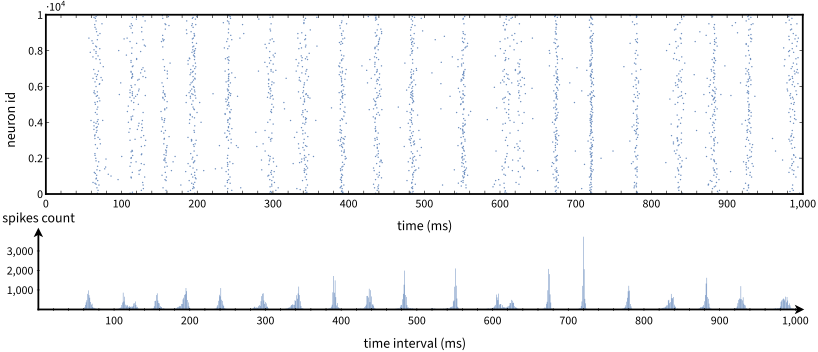
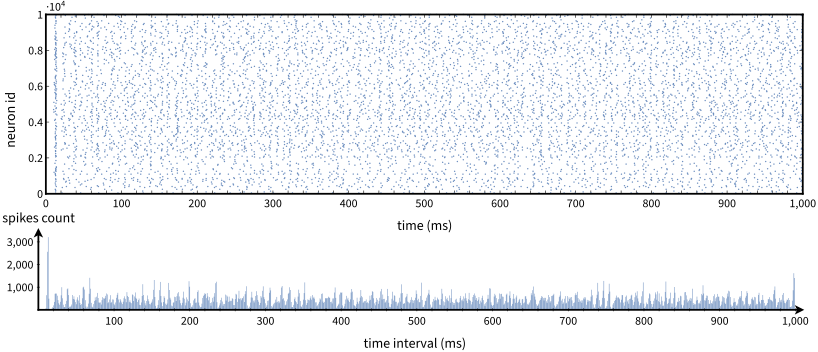
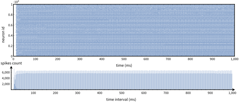
A C++-based Brunel network model of LIF neurons was implemented, and the appropriate stimuli were injected to reproduce three states of the original paper. Results are presented as a raster plot (a.k.a. spike trace, top), a timeline (left to right) of the spike times of the neurons, one row per neuron. Below it, a bar chart gives the number of neurons that spike in each interval of 1 ms.
Slow dynamics (SI slow):
Asynchronous dynamics (AI):
Synchronous regular dynamics (SR):
In the pictures above, the global activity oscillates slowly in the SI slow state, where each neuron fires irregularly at a very low rate. The network fires in bursts, at a global frequency of about 20 Hz, close to the 22 Hz of the simulation of the paper. With \(\eta = 0.9\), the external input alone keeps the mean potential under the threshold: the neurons fire only when the fluctuations of their input push them above it, so the first spikes come late.
The global activity is stationary in the AI state. In the SR state, the network is almost fully synchronized, and the neurons fire regularly at high rates: the spike count of the network repeats every 3 ms.
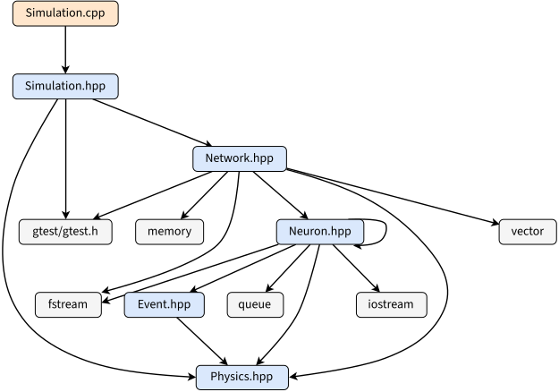
The C++ code can be downloaded as lif-brunel.tar.gz. To help understand the code, the include graph of Simulation.cpp is available in diagram_class.svg.