Roofline model and arithmetic intensity
The roofline model, presented in the 2009 paper Roofline: An Insightful Visual Performance Model for Multicore Architectures, shows whether a program is limited by compute or by memory bandwidth, and so which optimizations can make it faster. The model bounds the performance \(P\) of a program by its arithmetic intensity \(I\) (called operational intensity in the paper and in the picture below), the number of FLOPs it performs per byte that moves between memory and the processor. The bound is given by \(P \le \min(P_\text{peak}, B_\text{peak} \times I)\), where \(P_\text{peak}\) is the peak compute performance and \(B_\text{peak}\) the peak memory bandwidth of the hardware.
A roofline chart plots the attainable performance (GFLOPs/s) against the arithmetic intensity (FLOPs/byte), on a log-log scale, as in the following example with three applications:
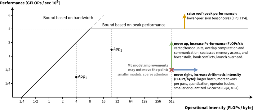
A roofline plot, on a log-log scale. App1 is memory-bound. App2 is compute-bound and runs below the peak performance. The arrows show how an application at ❌ moves right (more FLOPs per byte), moves up (closer to the roof), or gains from a higher roof.
The two terms of the minimum form a “roof”: a slanted line for the bandwidth bound and a flat line for the peak compute, which meet at the ridge point. A program to the left of the ridge point is memory-bound (e.g. a decode step), as the processor waits for data, and a program to its right is compute-bound (as prefill). The gap between a point and the roof is the performance lost to overheads, such as kernel launches, memory latencies or poor memory access patterns.
Moving right. A memory-bound point moves right, to more FLOPs per byte, where the roof is higher. A larger batch or more tokens per pass, e.g. batching and speculative decoding in decode, reuse each weight byte across more rows. Tiling in shared memory reuses the data, operator fusion avoids writing intermediates to HBM and reading them back, and quantization and smaller KV caches (GQA, MLA) read fewer bytes per FLOP, which matters most for decode.
Moving up. A point moves up, closer to the roof at the same intensity, with tensor cores and vectorized instructions, good occupancy and coalesced memory access. The roofline bound takes the slower of data movement and computation, as if they overlapped, and double buffering brings a program closer to it: the program computes on one tile while the next one loads into a second buffer, instead of alternating loads and computation. Fewer stalls help too: synchronization, bank conflicts, warp divergence and kernel launches, which CUDA graphs reduce for the many small kernels of decode.
Raising the roof. Compute-bound prefill is already near the flat roof. It gains from lower-precision tensor-core math, such as FP8 or FP4, which raises the roof, or from doing less work with sparse attention or smaller models, which cuts the runtime without necessarily moving the point.
How to draw the roofline of a GPU
To sketch the limits of a hardware architecture, two values are needed from the manufacturer’s specification sheet, for the chosen precision (e.g., FP32): the peak compute performance \(P_\text{peak}\), in GFLOPs/s, and the peak memory bandwidth \(B_\text{peak}\), in GB/s. With that, the ridge point, the arithmetic intensity at which the hardware shifts from being memory-bound to compute-bound, is then given by:
\[\text{Ridge Point} = \frac{\text{Peak Compute Performance } (P_{\text{peak}})}{\text{Peak Memory Bandwidth } (B_{\text{peak}})}\]At the left of the ridge point, the memory ceiling \(P = B_\text{peak} \times I\) is a line of slope 1 on the log-log scale, as \(\log P = \log B_\text{peak} + \log I\). At the right of it, the compute ceiling \(P = P_\text{peak}\) is flat.
How to calculate the roofline point for an application
To find the \(X\) coordinate of an application (❌ in the roofline plot above), the floating-point operations and the bytes moved are counted, e.g., by looking at the code or with hardware counters:
\[\text{Arithmetic Intensity } (X) = \frac{\text{Total FLOPs executed}}{\text{Total Bytes read and written}}\]To find the \(Y\) coordinate of ❌, the wall-clock execution time of the kernel is measured:
\[\text{Performance } (Y) = \frac{\text{Total FLOPs executed}}{\text{Execution Time (Seconds)} \times 10^9} \quad \text{[GFLOPs/s]}\]Example: 2D Vector sum
Consider a vector loop over \(N\) elements that computes \(C[i] = A[i] + B[i]\) with 32-bit single-precision floats (\(1 \text{ float} = 4 \text{ bytes}\)). It performs \(N\) additions and moves \(12N\) bytes, as it reads the arrays \(A\) and \(B\) and writes the array \(C\). Thus, its \(X\) coordinate is \(1/12 \approx 0.083\) FLOPs per byte, whatever \(N\), and its \(Y\) coordinate is \(N\) divided by its execution time, in GFLOPs/s.
At this intensity, the roof is the peak bandwidth divided by 12, far below the peak compute of any GPU. The vector sum is memory-bound: the best that an implementation can do is to move its data at the peak bandwidth.
Plotting the roofline
The following code plots the roofline of the A100 in FP32, and the point of the vector sum:
import matplotlib.pyplot as plt
import numpy as np

# 1. HARDWARE SPECS (e.g., NVIDIA A100 GPU)
P_peak = 19500  # Peak Compute: 19,500 GFLOPs/s
B_peak = 1555   # Peak Bandwidth: 1,555 GB/s
ridge_point = P_peak / B_peak  # ~12.54 FLOPs/byte

# 2. CODE SPECS (Vector Addition Example)
total_flops = 1_000_000                  # 1M additions
total_bytes = 1_000_000 * 3 * 4          # 3 arrays (A,B,C) of 4-byte floats
code_x = total_flops / total_bytes       # Arithmetic Intensity = FLOPs / Bytes = 0.083

# Performance = FLOPs / (Time * 1e9)
execution_time = 0.0001                  # 0.1 milliseconds
code_y = total_flops / (execution_time * 1e9)  # 10 GFLOPs/s

# 3. GENERATE ROOFLINE BOUNDARIES
x_line = np.logspace(-2, 3, 500)
y_line = np.minimum(P_peak, B_peak * x_line)

# 4. PLOT THE CHART
plt.figure(figsize=(8, 5))
plt.loglog(x_line, y_line, label="GPU Roofline Boundary", color="red", lw=2)
plt.scatter([code_x], [code_y], color="blue", s=100, zorder=5, label="Your Code")
plt.text(ridge_point * 1.2, P_peak * 0.7, f"Ridge Point: {ridge_point:.2f} FLOPs/B", color="red")
plt.text(code_x * 1.2, code_y, f"Your Code ({code_x:.3f}, {code_y:.1f})", color="blue")
plt.xlabel("Arithmetic Intensity (FLOPs/byte)")
plt.ylabel("Attainable Performance (GFLOPs/s)")
plt.title("Simple GPU Roofline Model Analysis")
plt.grid(True, which="both", ls="--")
plt.legend()
plt.savefig("simple_roofline.png") # Save the plot
plt.show()
Example: Matrix multiplication
Matrix multiplications perform most of the FLOPs of a transformer, in its projections, its MLP and its attention. For the multiplication of two matrices of shapes \(A \times B\) and \(B \times C\), which gives an output matrix of shape \(A \times C\), here are the FLOPs and the memory traffic, for a data type of \(dt\) bytes per element. Each element of the output is the dot product of a row of matrix 1 and a column of matrix 2, as illustrated in the following picture:
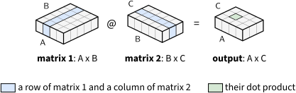
Step 1: Floating Point Operations (FLOPs). To compute each of the \(AC\) elements of the output matrix, a dot product of \(B\) multiplications and \(B\) additions is performed. Each multiply-accumulate counts as \(2\) FLOPs. Therefore:
\[\text{Total FLOPs} = 2ABC\]Step 2, naive: Memory Traffic (Bytes) without cache. The bytes loaded from memory depend on the implementation. If every element is fetched from main memory, without any reuse, matrix 1 is loaded \(C\) times (once per column of matrix 2), and matrix 2 is loaded \(A\) times (once per row of matrix 1), so \(2ABC\text{ }dt\) bytes are loaded.
Step 2, cache-optimized: Memory Traffic (Bytes) with cache. On a GPU, tiling loads the data into fast on-chip SRAM (shared memory or cache) and reuses it across many products. Each element of the inputs is then loaded once, and each element of the output written once, for a total of \((AB + BC + AC)\text{ }dt\) bytes.
Step 3: Arithmetic Intensity (Operational Intensity). Dividing the total FLOPs by the minimum memory traffic gives the arithmetic intensity (FLOPs per byte transferred):
\[\text{Arithmetic Intensity} = \frac{2ABC}{(AB + BC + AC)\text{ }dt}\]For large square matrices where \(A = B = C = N\), this simplifies to roughly \(\frac{2N}{3\text{ }dt}\) FLOPs per byte, making matrix multiplication compute-bound for large sizes and memory-bound for very small sizes.
Step 4: Roofline Coordinate. With the arithmetic intensity as X and the measured performance as Y, the point ❌ on the roofline model is:
\[(X, Y) = \left( \frac{2ABC}{(AB + BC + AC)\text{ }dt}, \; \frac{2ABC}{\text{Time}_{\text{sec}} \times 10^9} \right)\]Example: Tensor multiplication
For higher-dimensional tensors, e.g. with shapes \(A \times B \times D \times E \times F\) and \(B \times C \times D \times E \times F\), the extra dimensions act as batch axes: the tensor multiplication is a stack of \(DEF\) matrix multiplications, one per batch index, as illustrated in the following picture:
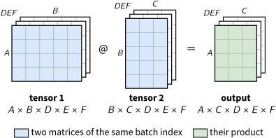
The FLOPs and the memory traffic both grow by the batch size \(DEF\), so the arithmetic intensity (X) is that of the 2D case, and only the performance (Y) is multiplied by \(DEF\):
\[(X, Y) = \left( \frac{2ABC}{(AB + BC + AC) \text{ } dt}, \; \frac{2ABC \text{ } DEF}{\text{Time}_{\text{sec}} \times 10^9} \right)\]Note that the extra dimensions keep the arithmetic intensity of a single matrix multiplication only because both tensors have them, as in attention, where every sequence and head multiplies its own queries, keys and values. In a decode step, each sequence reads its own keys and values from the KV cache, so attention performs about 1 FLOP per byte, whatever the batch size, or about as many as the query heads that share each key and value, with GQA. When matrix 2 is shared instead, as the weights of a linear layer are shared by all the sequences of a batch, the extra dimensions join \(A\), and the intensity grows with the batch. This is why batching speeds up the linear layers of decode, but not its attention.