Tensor parallelism like Megatron-LM
Tensor parallelism aims at partitioning computation across the model’s tensor dimensions (e.g., sharding linear layer weights and corresponding activations). This is a hard problem: in practice, the dimension of tensor partitioning (row-wise, column-wise, or none) must be decided, and the communication and computation adapted accordingly. Therefore, it is a model- and data-specific implementation. The following picture illustrates this partitioning on a small fully-connected network:
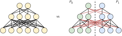
The previous picture shows a major drawback of this method: during training, processors need to continuously communicate the activations that are needed across the processor network. In the picture, half of the connections (the red ones) link neurons on different processors, as each neuron is connected to all the neurons of the next layer. With \(P\) processors, a fraction \({(P-1)/P}\) of the connections of every layer crosses processors. This communication is synchronous and can limit overlap with compute (depending on the implementation). And it can require a large amount of communication at every layer of the network and for every input batch.
There are several alternative ways to distribute multi-dimensional tensors across several compute nodes, which aim at reducing the number of communication steps or the communication volume. This post details and implements the Megatron-LM approach.
Megatron-LM tensor parallelism
Megatron-LM splits the two main blocks of a transformer layer, the feed-forward (MLP) and the attention block, so that the forward and the backward pass of each block need a single all-reduce: two all-reduces in the forward pass and two in the backward pass of each layer. The two blocks, split over two GPUs, are illustrated in the following picture (Figure 3 in the paper):
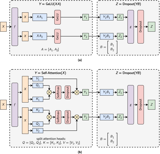
(a) The MLP block and (b) the self-attention block of Megatron-LM, split over two GPUs: the first weight matrix \(A\) is split by columns (\(Q\), \(K\) and \(V\) by attention heads), and the second one, \(B\), by rows. \(f\) and \(g\) are conjugate operators: \(f\) is an identity operator in the forward pass and an all-reduce in the backward pass, while \(g\) is an all-reduce in the forward pass and an identity in the backward pass. Adapted from: Megatron-LM: Training Multi-Billion Parameter Language Models Using Model Parallelism
The MLP block: column-parallel and row-parallel linear layers
The MLP is a sequence of a matrix multiplication (MatMul) \(XA\), an activation function \(\phi\), a GeLU (Gaussian Error Linear Unit) in Megatron-LM, whose output is \(Y = \phi(XA)\), a second MatMul \(Z = YB\) and a dropout, where \(X\) is the input, with one row per token, and \(A\) and \(B\) are the weight matrices of the two linear layers. Megatron-LM splits the two MatMuls across GPUs in two steps:
- The first MatMul keeps \(X\) whole on every GPU and splits \(A\) by columns, so each GPU computes its own columns of \(Y\), \([Y_1, Y_2] = [\phi(X A_1), \phi(X A_2)]\), without any communication. Splitting \(A\) by rows (and \(X\) by columns) instead would need a sum before \(\phi\), as \(\phi\) is nonlinear.
- The second MatMul splits \(B\) by rows, to match the columns of \(Y\) on each GPU, so each GPU computes a partial sum \(Y_i B_i\), and an all-reduce adds them up into \(Z = Y_1 B_1 + Y_2 B_2\).
Therefore, the two MatMuls need a single communication step, as illustrated below:
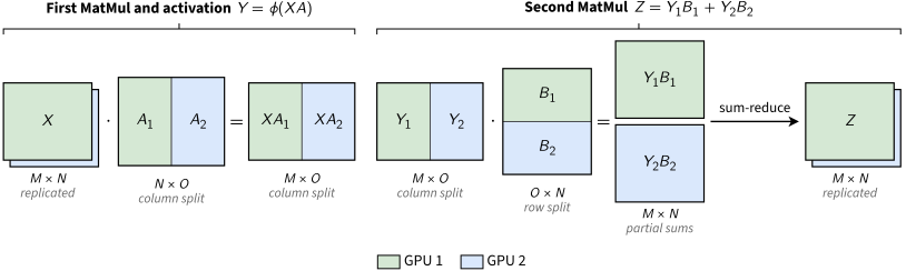
The two linear layers of the MLP are named after the split of their weights: the first one is column-parallel, as each GPU holds some of the columns of \(A\), and the second one is row-parallel, as each GPU holds some of the rows of \(B\). A column-parallel layer takes a replicated input and gives an output split by columns, and a row-parallel layer takes an input split by columns and gives partial sums that must be added.
The operators f and g
Megatron-LM makes this implementation very simple, by adding only the \(f\) and \(g\) functions to the serial use case. Following the paper: “\(f\) is an identity operator in the forward pass and all reduce in the backward pass while \(g\) is an all reduce in the forward pass and identity in the backward pass”.
In the forward pass, every GPU reads the same input \(X\), so \(f\) does nothing, and \(g\) adds the partial sums \(Y_1 B_1\) and \(Y_2 B_2\). In the backward pass, each GPU computes only the part of the gradient of \(X\) that comes from its own columns of \(A\), so \(f\) adds these parts, and \(g\) does nothing. In brief, the backward pass of a copy is a sum, and the backward pass of a sum is a copy. In PyTorch, each of them is an autograd function:
class Megatron_f(torch.autograd.Function):
  """ The f function in Figure 3 in Megatron paper """

  @staticmethod
  def forward(ctx, x, mp_comm_group=None):
      ctx.mp_comm_group = mp_comm_group
      return x

  @staticmethod
  def backward(ctx, gradient):
      dist.all_reduce(gradient, dist.ReduceOp.SUM, group=ctx.mp_comm_group)
      return gradient, None
and
class Megatron_g(torch.autograd.Function):
  """ The g function in Figure 3 in Megatron paper """

  @staticmethod
  def forward(ctx, x, mp_comm_group=None):
      dist.all_reduce(x, dist.ReduceOp.SUM, group=mp_comm_group)
      return x

  @staticmethod
  def backward(ctx, gradient):
      return gradient, None
The argument mp_comm_group is the model-parallel communication group, which allows tensor parallelism to be combined with other types of parallelism. The MLP then calls \(f\) at the start of the block and \(g\) at its end, as in the paper, where n_embd_mid is the hidden size on each GPU, \(4E/P\):
class Megatron_FeedForward(nn.Module):
  """ the feed forward network (FFN) in the paper, with tensor parallelism as in Megatron-LM MLP block"""

  def __init__(self, n_embd, mp_comm_group=None):
    super().__init__()
    self.mp_comm_group = mp_comm_group

    #Fig 3a. MLP: splits first GEMM across columns and second GEMM across rows
    n_embd_mid = n_embd * 4
    if self.mp_comm_group:
        n_embd_mid //= dist.get_world_size(group=self.mp_comm_group)

    self.fc1 = nn.Linear(n_embd, n_embd_mid)
    self.fc2 = nn.Linear(n_embd_mid, n_embd, bias=False)   # <-- no bias here
    self.fc2_bias = nn.Parameter(torch.zeros(n_embd))      # <-- bias added after all-reduce
    self.dropout = nn.Dropout(dropout)

  def forward(self, x):
    if self.mp_comm_group:
        x = Megatron_f.apply(x, self.mp_comm_group)

    y = F.gelu(self.fc1(x))

    z = self.fc2(y)  # matmul only (partial)

    if self.mp_comm_group:
        z = Megatron_g.apply(z, self.mp_comm_group)

    z = z + self.fc2_bias  # <-- bias AFTER all-reduce
    z = self.dropout(z)
    return z
Note that the all-reduce of \(g\) comes before the bias of the second linear layer, as otherwise the bias would be added once per GPU.
The attention block
The algorithm of the attention mechanism is analogous, except that instead of a single MatMul \(XA\) at the beginning of the workflow, there are three MatMuls \(XV\), \(XQ\) and \(XK\) for the value, query and key matrices. Therefore, the attention block also requires one (not two) communication step, as the MLP block. Its parts are split as follows:
- The Q, K and V projections are column-parallel: their output features (the heads) are split, so each GPU (a rank, in the code) owns a subset of the heads.
- The attention softmax is computed locally on each GPU, because the heads are independent of each other.
- The output projection is row-parallel, and that is where the all-reduce of \(g\) is done, to add up the partial outputs of the GPUs.
The multi-head attention block can then be written as follows, where B, S and E are the batch size, the sequence length and the embedding size (this B is not the weight matrix \(B\) of the MLP):
class Megatron_MHA(nn.Module):
  """ Megatron-LM MHA: column-parallel Q/K/V, row-parallel output projection """

  def __init__(self, n_embd, n_head, block_size, dropout, mp_comm_group=None):
    super().__init__()
    self.mp_comm_group = mp_comm_group
    self.n_embd = n_embd
    self.n_head = n_head

    self.tp_size = dist.get_world_size(group=mp_comm_group) if mp_comm_group else 1
    if n_head % self.tp_size != 0:
      raise ValueError(f"n_head ({n_head}) must be divisible by tp_size ({self.tp_size}).")

    self.n_head_local = n_head // self.tp_size

    if n_embd % n_head != 0:
      raise ValueError(f"n_embd ({n_embd}) must be divisible by n_head ({n_head}).")
    self.head_dim = n_embd // n_head
    self.hidden_local = self.n_head_local * self.head_dim

    # Column-parallel QKV: each rank produces Q,K,V only for its local heads.
    self.qkv = nn.Linear(n_embd, 3 * self.hidden_local, bias=False)

    # Row-parallel output projection: consumes local heads and produces full n_embd,
    # then we all-reduce (Megatron_g) to combine ranks.
    self.proj = nn.Linear(self.hidden_local, n_embd, bias=False)

    self.register_buffer("tril", torch.tril(torch.ones(block_size, block_size)))
    self.attn_dropout = nn.Dropout(dropout)
    self.out_dropout = nn.Dropout(dropout)

  def forward(self, x):
    B, S, E = x.shape
    if E != self.n_embd:
      raise ValueError(f"Expected x.shape[-1] == {self.n_embd}, got {E}.")

    # Column-parallel input handling: identity forward, all-reduce on backward.
    if self.mp_comm_group:
      x = Megatron_f.apply(x, self.mp_comm_group)

    # Local QKV for local heads
    qkv = self.qkv(x)  # (B, S, 3*hidden_local)
    q, k, v = qkv.split(self.hidden_local, dim=-1)

    # (B, S, hidden_local) -> (B, n_head_local, S, head_dim)
    q = q.view(B, S, self.n_head_local, self.head_dim).transpose(1, 2)
    k = k.view(B, S, self.n_head_local, self.head_dim).transpose(1, 2)
    v = v.view(B, S, self.n_head_local, self.head_dim).transpose(1, 2)

    # Attention scores: (B, n_head_local, S, S)  -- LOCAL, no comm
    wei = (q @ k.transpose(-2, -1)) * (self.head_dim ** -0.5)

    # Causal mask (broadcasts over B and n_head_local)
    wei = wei.masked_fill(self.tril[:S, :S] == 0, float("-inf"))

    wei = F.softmax(wei, dim=-1)
    wei = self.attn_dropout(wei)

    # Context: (B, n_head_local, S, head_dim)
    out = wei @ v

    # Concat heads: (B, S, hidden_local)
    out = out.transpose(1, 2).contiguous().view(B, S, self.hidden_local)

    # Row-parallel output projection: local matmul then all-reduce sum on forward
    out = self.proj(out)  # (B, S, n_embd) partial contribution
    if self.mp_comm_group:
      out = Megatron_g.apply(out, self.mp_comm_group)

    out = self.out_dropout(out)
    return out
In a more recent attention module, Multi-Head Latent Attention, the keys and values of all heads come from one latent vector per token, so every GPU needs all of it. Tensor Parallel Latent Attention (TPLA) splits this latent vector across the GPUs too.
Sharding activations for further memory saving
The main caveat of this method is that the input X of each block and the activations of the layer normalizations and dropouts between blocks are replicated across all GPUs. Sequence parallelism shards them along the sequence dimension, as these operations treat each token independently. It does so by replacing the all-reduce at the end of each block (every second layer) with an all-gather at the start of the block and a reduce-scatter at its end, which swap roles in the backward pass. Each GPU then stores only \(1/P\) of these activations.
Detour: spatial parallelism on Convolutional Neural Nets
Spatial parallelism extends tensor parallelism to convolutional layers. In this example, the activations of a 2D input are split across processors along their height and width. As a convolution filter has a short spatial span, each processor computes the convolution of its part on its own, and exchanges only the activations at the boundaries of its part, the halo region, as illustrated below:
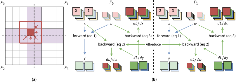
Two ways to parallelize a convolutional neural network. (a) Spatial parallelism: the activations of a 2D input are split across four processors \(P_0\) to \(P_3\). The red box is where the 3x3 convolution filter is centered, the red arrows are the data that must be received from the other processors to compute it, and the purple region is the halo, formed by all the elements exchanged at every step. (b) Sample (data) parallelism on two processors \(P_0\) and \(P_1\), with a global mini-batch of 4 samples. Blue arrows are the dependencies of the forward pass, which computes the output \(y\) from the input \(x\) and the filters \(w\); green arrows are those of the backward pass, which computes the gradients of the filters, \(dL/dw\), and of the input, \(dL/dx\), from \(dL/dy\). The labels eq 1 to eq 3 refer to the equations of the paper. The only communication between \(P_0\) and \(P_1\) is the all-reduce of \(dL/dw\). Adapted from: Improving Strong-Scaling of CNN Training by Exploiting Finer-Grained Parallelism