Unsupervised Learning for Clustering
Unsupervised learning is the field of machine learning dedicated to learning without supervision or reward signals. Its methods are commonly used to group similar data, to compress it, and to visualize it. This post details a few of the most common clustering methods, each with a short NumPy implementation.
Clustering
Clustering groups the data points so that the points of a group, a cluster, are more similar to each other than to the points of other clusters. As there are no labels, each method has its own definition of a cluster: the points closest to a prototype (k-means), a branch of a tree (hierarchical clustering) or a dense region of points (DBSCAN).
K-Means
A common technique for data reduction is prototype clustering, where the data points \(x_u\) are represented by a smaller set of prototypes \(w_i\), one per cluster of points. The general rule is that a new point \(x\) belongs to the closest prototype \(i^*\), i.e.
\[\| w_{i^*} - x \| \leq \| w_i - x \| \text{, for all } i\]The reconstruction (squared) error is the sum of the errors of all data points over all clusters \(C_i\):
\[E = \sum_{i=1}^{k} \sum_{u \in C_i} \| w_i - x_u \|^2\]k-means clustering is an iterative method for prototype clustering. It looks for the partition of the data points into \(k\) clusters that minimizes this error, where each prototype \(w_i\) is the mean of the points of its cluster. The standard algorithm, also called Lloyd’s algorithm, alternates between two steps:
- assignment step: assign each point to the closest mean, e.g. in Euclidean distance;
- update step: move each mean to the centroid of the points of its cluster:
The algorithm converges when the assignments no longer change. With the update \(\Delta w_i = \eta \sum_{u \in C_i} (x_u - w_i)\), convergence means \(\Delta w_i = 0\), so it must hold that:
\[\eta \sum_{u \in C_i} (x_u - w_i) = 0 \rightarrow \sum_{u \in C_i} x_u - \vert C_i \vert \, w_i =0 \rightarrow w_i = \frac{1}{\vert C_i \vert} \sum_{u \in C_i} x_u\]which is the center of mass of cluster \(i\). Neither step increases the error, and there is a finite number of partitions, so k-means always converges, but possibly to a local minimum. Thus, it is usually run several times from different initial means, e.g. picked far from each other with k-means++. An illustration of the algorithm follows:
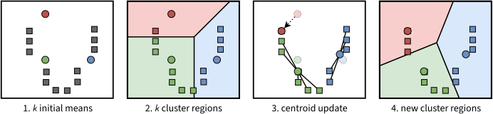
1. \(k = 3\) initial means (colored circles) are chosen at random. 2. Assignment step: each point joins the cluster of the closest mean; the colored regions are the Voronoi cells of the means. 3. Update step: each mean moves to the centroid of its cluster (dashed circles: the previous means). 4. Assignment step with the new means. The two steps repeat until the assignments no longer change. Adapted from: k-means clustering
A whole run of k-means on 2D data is illustrated below:
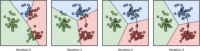
Iterations of k-means with \(k = 3\) on three Gaussian clusters. Each panel shows the means (circles), their Voronoi cells and their clusters, and the lines trace the previous means. Two initial means start in the same cluster, and one of them moves down to the cluster that has no mean.
The following function picks \(k\) data points at random as the initial means, and returns the means and the cluster of each point. A cluster that loses all its points keeps its mean, as the centroid of an empty cluster is not defined:
import numpy as np

def kmeans(X, k, steps=100, seed=0):
    rng = np.random.default_rng(seed)
    W = X[rng.choice(len(X), k, replace=False)]  # k data points as the initial means
    for _ in range(steps):
        labels = ((X[:, None] - W) ** 2).sum(2).argmin(1)  # assignment step
        new = np.array([X[labels == i].mean(0) if np.any(labels == i) else W[i]
                        for i in range(k)])  # update step
        if np.allclose(new, W):  # the means, and thus the assignments, no longer change
            break
        W = new
    return W, labels
The update \(\Delta w_i\) above is a batch learning rule, as it updates the weights with a set (batch) of inputs. The online update rule, instead, updates the winning prototype \(i\) at every new input \(x_u\), as the self-organizing maps below do:
\[\Delta w_i = \eta (x_u - w_i)\]K-Nearest Neighbors
The k-nearest neighbors algorithm (KNN) is not to be confused with k-means. It is not a clustering method either: it is a supervised classifier, as it needs the labels of the training points. It is covered here because its core operation, finding the \(k\) points closest to a query, is the building block of many unsupervised methods.
Given a query point \(x\), KNN finds the \(k\) training points closest to it, and predicts the most common label among them (classification), or the average of their values (regression). There is no training step: the model is the training set itself. A small \(k\) follows the training data closely and is sensitive to noise, while a large \(k\) gives smoother boundaries between classes, as in the picture below. In practice, \(k\) is chosen by cross-validation, and an odd \(k\) avoids ties between two classes.
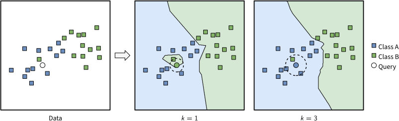
KNN in 2D, with the training points of class A (blue) and class B (green), and a query point (circle) next to a single point of B among the points of A. The colored regions show the class that KNN predicts at each position, and the dashed circle holds the \(k\) nearest neighbors of the query. With \(k = 1\), the query takes the label B of its nearest neighbor; with \(k = 3\), its neighbors vote A, and the boundary between the classes is smoother.
The following function implements a KNN classifier:
def knn(X, y, x, k):
    nearest = np.argsort(((X - x) ** 2).sum(1))[:k]  # the k points closest to x
    labels, votes = np.unique(y[nearest], return_counts=True)
    return labels[votes.argmax()]  # the most common label among them
This brute-force search computes the distances from the query to all \(n\) training points, i.e. \(O(nd)\) operations per query in \(d\) dimensions. Also, the distances must be meaningful: the features are usually normalized first, so that a feature with a large range does not dominate the distance.
The Curse of Dimensionality
A faster search would skip the points that are far from the query. However, the spatial indexes of databases, such as k-d trees, do not help in high dimensions, due to the curse of dimensionality: as the number of dimensions grows, the nearest and the farthest neighbors of a point end up at almost the same distance. The squared distance between two points is a sum of one term per dimension: its mean grows with the number of dimensions \(d\), while its spread grows only with \(\sqrt{d}\). The following picture shows how the distances concentrate around their mean:
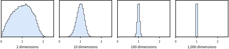
Histograms of the distances from random query points to points drawn uniformly in the unit cube, each divided by the mean distance from its query point. In 2 dimensions, the distances range from almost 0 to twice the mean, while in 1,000 dimensions they are all close to the mean.
A k-d tree splits the space with one axis-aligned plane per node, so that a query visits only the regions near it. In high dimensions, all regions are about as close to the query, and the search visits almost all of them. Real data, however, often lies close to a surface of much lower dimension than its number of coordinates, so the nearest neighbors of a point still stand out, and KNN still works on it.
Hierarchical Clustering
Hierarchical clustering builds a tree of clusters (a dendrogram) instead of a single partition. Its common agglomerative (bottom-up) variant starts with one cluster per data point, and repeatedly merges the two closest clusters, until a single cluster remains. The distance between two clusters \(A\) and \(B\) is given by the linkage criterion:
- single linkage: the distance between their closest points, \(\min_{a \in A, b \in B} d(a,b)\). It finds elongated clusters, but can chain distinct clusters together through a few close points;
- complete linkage: the distance between their farthest points, \(\max_{a \in A, b \in B} d(a,b)\), which favors compact clusters;
- average linkage: the average distance between all pairs of points, \(\frac{1}{\vert A \vert \vert B \vert} \sum_{a \in A} \sum_{b \in B} d(a,b)\);
- Ward’s linkage: the increase of the k-means error caused by merging \(A\) and \(B\), which is \(\frac{\vert A \vert \vert B \vert}{\vert A \vert + \vert B \vert} \| \mu_A - \mu_B \|^2\) for the cluster means \(\mu_A\) and \(\mu_B\).
Cutting the dendrogram at a given height yields a partition, so the number of clusters can be chosen after the fact, by looking at the tree:
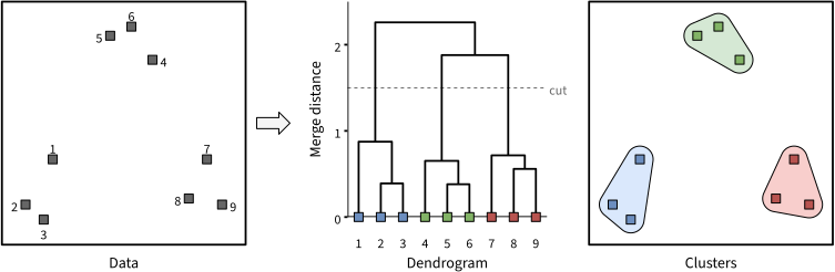
Single linkage on nine points in 2D, numbered in the order of the leaves of the dendrogram. The close points of each group merge first, and the three groups join last. A cut at a height of 1.5 (dashed line) gives three clusters, drawn on the right.
The divisive (top-down) variant does the opposite: it starts with all points in one cluster, and splits clusters recursively. Agglomerative clustering needs the \(n \times n\) matrix of pairwise distances, and runs in \(O(n^2)\) to \(O(n^3)\) time, so it suits small to medium datasets.
The following function implements agglomerative clustering. The linkage is a function of the distances between the points of two clusters: np.min for single linkage, np.max for complete linkage and np.mean for average linkage. The function returns the merges, each with its two clusters and its height:
def agglomerative(X, link=np.min):
    D = np.sqrt(((X[:, None] - X) ** 2).sum(2))  # the distances between all points
    clusters, merges = [[i] for i in range(len(X))], []
    while len(clusters) > 1:  # merge the two closest clusters, a and b
        n = len(clusters)
        h, a, b = min((link(D[np.ix_(clusters[a], clusters[b])]), a, b)
                      for a in range(n) for b in range(a + 1, n))
        merges.append((clusters[a], clusters[b], float(h)))
        clusters[a] = clusters[a] + clusters.pop(b)
    return merges
DBSCAN
DBSCAN (Density-Based Spatial Clustering of Applications with Noise) defines clusters as dense regions separated by sparse ones. It takes two parameters, a radius \(\varepsilon\) and a minimum number of points \(m\), and labels each point as:
- a core point, if at least \(m\) points (itself included) lie within distance \(\varepsilon\) of it;
- a border point, if it is not a core point but lies within distance \(\varepsilon\) of a core point;
- noise, otherwise.
Two core points within distance \(\varepsilon\) of each other belong to the same cluster, so each cluster is a connected group of core points, plus the border points around them. Unlike k-means, DBSCAN does not need the number of clusters, finds clusters of any shape, and labels outliers as noise. However, a single radius \(\varepsilon\) cannot capture clusters of very different densities, a limitation addressed by its extensions OPTICS and HDBSCAN.
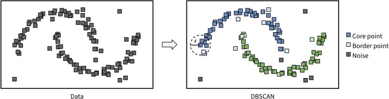
DBSCAN, with \(\varepsilon = 0.25\) and \(m = 6\), on two half-moons and uniform noise. The dashed circle shows the radius \(\varepsilon\) around a core point. DBSCAN finds the two moons as two clusters, blue and green, with dark core points and light border points, and labels the isolated points as noise (grey).
The following function implements DBSCAN, and labels the noise \(-1\). It grows each cluster from a core point that is not yet in a cluster, with a stack of the core points whose neighbors remain to be visited:
def dbscan(X, eps, m):
    D = np.sqrt(((X[:, None] - X) ** 2).sum(2))
    neighbors = [np.flatnonzero(d <= eps) for d in D]  # within eps, itself included
    core = [len(nb) >= m for nb in neighbors]
    labels, c = np.full(len(X), -1), 0  # -1 marks the noise, c is the next cluster
    for p in range(len(X)):
        if core[p] and labels[p] == -1:  # a new cluster, grown from the core point p
            labels[p], stack = c, [p]
            while stack:
                for q in neighbors[stack.pop()]:
                    if labels[q] == -1:
                        labels[q] = c
                        if core[q]:  # only core points extend the cluster
                            stack.append(q)
            c += 1
    return labels
Spectral Clustering
Spectral clustering treats clustering as a graph partitioning problem. It builds a graph of the data points, with a similarity \(W_{ij}\) for each pair of points, e.g. \(W_{ij} = \exp ( - \| x_i - x_j \|^2 / 2\sigma^2 )\) between each point and its nearest neighbors and \(0\) otherwise, and looks for clusters connected by edges of little weight. With the degree matrix \(D\), a diagonal matrix with \(D_{ii} = \sum_j W_{ij}\), the graph Laplacian is \(L = D - W\), and for any vector \(f\):
\[f^T L f = \frac{1}{2} \sum_{i,j} W_{ij} (f_i - f_j)^2\]So \(f^T L f\) is small when \(f\) takes similar values on strongly connected points, and the eigenvectors of \(L\) with the smallest eigenvalues vary little within clusters. The algorithm is:
- compute the eigenvectors \(u_1, ..., u_k\) of the \(k\) smallest eigenvalues of \(L\), or of the normalized Laplacian \(L_{sym} = I - D^{-1/2} W D^{-1/2}\), usually preferred, as its cut also keeps the points of each cluster strongly connected, and not only the clusters apart;
- stack them as the columns of an \(n \times k\) matrix \(H\), and take its \(i\)-th row as the new \(k\)-dimensional representation of point \(x_i\) (with \(L_{sym}\), after normalizing each row to unit length);
- cluster the rows of \(H\) with k-means.
Spectral clustering separates non-convex clusters that k-means cannot, as the two rings of the picture below, at the cost of an eigendecomposition of an \(n \times n\) (sparse) matrix:
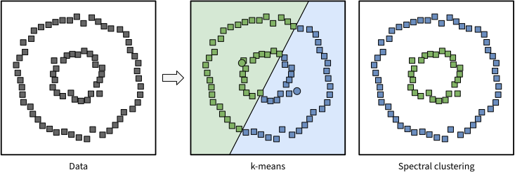
Two concentric rings, clustered by k-means (center), with the Voronoi cells of its two means, and by spectral clustering on the graph of the 8 nearest neighbors of each point (right). K-means cuts both rings in halves, while spectral clustering separates the rings.
The following function implements spectral clustering with the normalized Laplacian \(L_{sym}\), where an edge joins each point to its nearest neighbors, and clusters the rows of \(H\) with the kmeans function above:
def spectral_clustering(X, k, neighbors=8, sigma=1.0):
    D2 = ((X[:, None] - X) ** 2).sum(2)
    W = np.exp(-D2 / (2 * sigma**2))
    far = D2 > np.sort(D2, 1)[:, [neighbors]]  # not among the nearest neighbors
    W[far & far.T] = 0  # an edge joins each point to its nearest neighbors
    np.fill_diagonal(W, 0)
    d = W.sum(1)  # the degrees
    L = np.eye(len(X)) - W / np.sqrt(np.outer(d, d))  # L_sym = I - D^-1/2 W D^-1/2
    H = np.linalg.eigh(L)[1][:, :k]  # the eigenvectors of the k smallest eigenvalues
    H /= np.sqrt((H ** 2).sum(1, keepdims=True))  # rows of unit length
    return kmeans(H, k)[1]
Gaussian Mixture Models
K-means has two main problems:
- it forces the clusters to be spherical, while elliptical clusters are sometimes a better fit;
- each point belongs to one cluster only, which is not always a good choice for the points between two clusters.
Both problems are solved by Gaussian mixture models. A Gaussian mixture model (GMM) describes the data as drawn from \(K\) Gaussians: each data point picks a component \(k\) with probability \(\pi_k\), and is then drawn from the Gaussian \(\mathcal{N}(\mu_k, \Sigma_k)\), so that:
\[p(x) = \sum_{k=1}^K \pi_k \, \mathcal{N}(x \mid \mu_k, \Sigma_k), \text{ with } \sum_{k=1}^K \pi_k = 1.\]The covariance matrices \(\Sigma_k\) give each cluster an elliptical shape, and each point belongs to every cluster with some probability. The parameters maximize the log-likelihood \(\sum_{i=1}^n \log p(x_i)\) of the \(n\) data points, and are learned with the Expectation-Maximization (EM) algorithm, which alternates two steps, like k-means:
- E-step: compute the responsibility of each component \(k\) for each point \(x_i\), i.e. the probability that \(x_i\) was drawn from it:
- M-step: update the parameters, with the responsibilities as weights, where \(n_k = \sum_{i} \gamma_{ik}\) is the effective number of points of component \(k\):
Each iteration never decreases the log-likelihood, and EM converges to a local maximum. So, as k-means, it is run from several initializations, or initialized with the result of k-means. In fact, k-means is a limit case of EM: for a GMM whose components share the covariance \(\sigma^2 I\), the responsibilities become hard assignments to the closest mean as \(\sigma \rightarrow 0\). In practice, k-means is cheaper and suits large datasets with compact clusters, while a GMM suits elliptical or overlapping clusters:
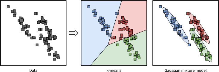
Three elongated clusters, clustered by k-means (center), with the Voronoi cells of its three means, and by a GMM (right), with the contour at two standard deviations of each Gaussian. The Voronoi cells of k-means cut across the clusters, while the ellipses of the GMM follow them.
The following function fits a GMM with EM, starting from the means of k-means, and returns the weights \(\pi_k\), the means \(\mu_k\), the covariance matrices \(\Sigma_k\) and the responsibilities \(\gamma_{ik}\). The cluster of each point is the component of largest responsibility, gamma.argmax(1):
def gmm(X, K, steps=100, seed=0):
    n, d = X.shape
    mu = kmeans(X, K, seed=seed)[0]  # the means of k-means as the initial means
    Sigma = np.array([np.diag(X.var(0))] * K)  # the variances of the data
    pi = np.full(K, 1 / K)
    for _ in range(steps):
        diff = X[:, None] - mu  # x_i - mu_k, for each point i and component k
        # pi_k N(x_i | mu_k, Sigma_k), with the squared Mahalanobis distances
        maha = np.einsum('ikd,kde,ike->ik', diff, np.linalg.inv(Sigma), diff)
        p = pi * np.exp(-maha / 2) / np.sqrt(np.linalg.det(2 * np.pi * Sigma))
        gamma = p / p.sum(1, keepdims=True)  # E-step: the responsibilities
        nk = gamma.sum(0)  # M-step
        mu = gamma.T @ X / nk[:, None]
        diff = X[:, None] - mu
        Sigma = np.einsum('ik,ikd,ike->kde', gamma, diff, diff) / nk[:, None, None]
        Sigma += 1e-6 * np.eye(d)  # keeps each covariance matrix invertible
        pi = nk / n
    return pi, mu, Sigma, gamma
Self-Organizing Maps
A self-organizing map (SOM), or Kohonen map, is an unsupervised neural network, typically a 2D grid of neurons, introduced by Teuvo Kohonen in 1982. The weights of each neuron are a point of the input space, a prototype as in k-means, that represents a region of similar inputs. Unlike k-means, the prototypes are ordered on a grid: neighboring neurons represent nearby regions of the input space.
The algorithm is the following:
- the weights of the neurons are initialized at random in the input space;
- at every iteration, choose an input \(x_u\);
- find the winner (or best matching unit) \(j^*\), the closest neuron:
- update the weights of the winner and of its neighbors, by pulling them closer to the input:
where \(h(j, j^*)\) is the neighborhood function, which decreases with the distance between neurons \(j\) and \(j^*\) in the grid (e.g. a Gaussian). If \(h\) is \(1\) for the winner and \(0\) for all other neurons, this is the online update rule of k-means. It is also common to decrease \(\eta\) and the width of \(h\) as the iterations progress;
- repeat until the weights no longer change, or for a maximum number of iterations.
The following picture illustrates the training of a SOM on 2D inputs:
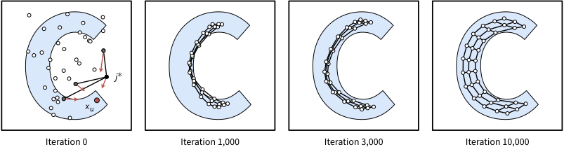
A SOM of 3x12 neurons, trained on 2D inputs drawn from the letter C (blue). Each circle is the weight vector of a neuron, and the lines join the neurons that are neighbors in the grid. The first panel shows the first update: the input \(x_u\) (red) selects the winner \(j^*\) (black), and the winner and its neighbors in the grid (grey) move towards \(x_u\) (red arrows). The weights start at random, then order themselves into a strip, which spreads until it covers the letter.
The following function implements the algorithm on a grid of size x size neurons, with a constant \(\eta\) and a Gaussian \(h\) of constant width, and returns the weight vector of each neuron:
def som(X, size=6, steps=10000, eta=0.2, width=1.0, seed=0):
    rng = np.random.default_rng(seed)
    grid = np.indices((size, size)).reshape(2, -1).T  # the position of each neuron
    W = rng.uniform(X.min(), X.max(), (size * size, X.shape[1]))  # random weights
    for x in X[rng.permutation(np.arange(steps) % len(X))]:  # in a random order
        winner = ((W - x) ** 2).sum(1).argmin()  # the best matching unit j*
        h = np.exp(-((grid - grid[winner]) ** 2).sum(1) / (2 * width**2))  # h(j, j*)
        W += eta * h[:, None] * (x - W)
    return W
A good example is the clustering of the handwritten digits of the MNIST database. Each digit is a 28x28 image, i.e. a point in 784 dimensions, and so is the weight vector of each neuron, which can be drawn as an image. The following picture shows three SOMs trained on the digits 0 to 3:
- left: a well-tuned SOM,
som(X), where each quadrant of neurons represents a digit; - center: a high learning rate,
som(X, eta=0.9), makes the neurons jump over long distances, and mixes the digits on nearby neurons; - right: a large neighborhood width,
som(X, width=4), makes all neurons move together, so that they all learn similar images.
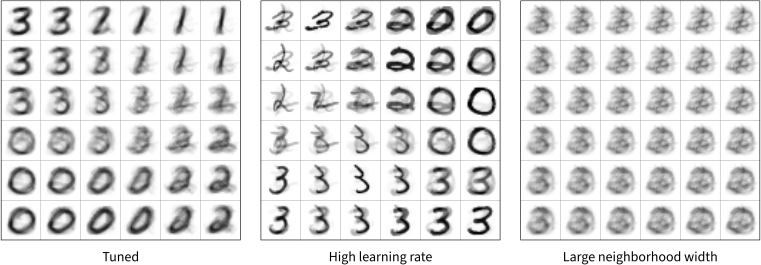
SOMs of 6x6 neurons, trained on the digits 0 to 3, with each neuron drawn as the 28x28 image of its weights.
Comparison of the Clustering Methods
The following table sums up the clustering methods of this section:
| Method | A cluster is | Number of clusters | When to use it |
|---|---|---|---|
| k-means | The points closest to a mean | Given, \(k\) | Large datasets with compact, spherical clusters |
| Hierarchical | A branch of the dendrogram | Chosen after the fact, by cutting the tree | Small to medium datasets, nested clusters |
| DBSCAN | A connected group of core points, plus their border points | Found by the method | Clusters of any shape, with similar densities, and outliers |
| Spectral | A group of strongly connected points of the similarity graph | Given, \(k\) | Non-convex clusters, e.g. two concentric rings |
| Gaussian mixture | A Gaussian of the mixture, with soft assignments | Given, \(K\) | Elliptical or overlapping clusters |
| Self-organizing map | The inputs closest to a neuron of the grid | The neurons of the grid | A 2D map of the data, where nearby neurons represent nearby inputs |