Unsupervised Learning basics and Principal Component Analysis
In 1901, Karl Pearson described the method known today as principal component analysis, in the paper On lines and planes of closest fit to systems of points in space. In 1957, Stuart Lloyd proposed the algorithm known today as k-means, to quantize signals, although his paper Least squares quantization in PCM was only published in 1982.
Unsupervised learning is the field of machine learning dedicated to learning without supervision or reward signals. Unlike reinforcement learning and supervised learning, the data is the only information given to the method. Still, these methods are very powerful, and are commonly used for image compression, dimensionality reduction, clustering and visualization, and to learn representations of the data that other models then build on. This post covers Hebbian learning, principal and independent component analysis (PCA and ICA), clustering methods (k-means, Gaussian mixtures, hierarchical clustering, DBSCAN and spectral clustering), self-organizing maps, t-SNE and UMAP, and autoencoders and self-supervised learning.
Foreword: Hebbian Learning
Among the many biologically inspired learning models, Hebbian learning (Donald Hebb, 1949) is probably the oldest. Its principle underlies many unsupervised learning rules, including several in this post. It is based on the synaptic changes between neurons that spike at close instants in time (motto: “if they fire together, they wire together”).
Spike-Timing-Dependent Plasticity (STDP, Markram et al., Frontiers) shows that the increase or decrease of the strength of a synapse depends on the time difference between the spikes of the pre- and the post-synaptic neurons. In essence, if a neuron spikes and leads to the firing of the output neuron, the synapse between them is strengthened.
In Hebb’s own words (1949):
When an axon of cell A is near enough to excite a cell B and repeatedly or persistently takes part in firing it, some growth process or metabolic change takes place in one or both cells such that A’s efficiency, as one of the cells firing B, is increased.
Analogously, in artificial systems, the weight of the connection between two artificial neurons adapts in the same way. Mathematically, the change over time of the weight \(w_{ij}\), from a pre-synaptic neuron \(i\) with activity \(x_i\) to a post-synaptic neuron \(j\) with output \(y_j\), can be described with the general Hebb’s rule:
\[\frac{d}{dt}w_{ij} = F (w_{ij}; x_i, y_j)\]or with the simplest Hebbian learning rule:
\[\frac{d}{dt}w_{ij} = \eta \, x_i \, y_j\]where \(\eta\) is the learning rate. Hebbian learning is local, i.e. it only looks at the two neurons involved, and ignores the activity of the rest of the system. It is a form of unsupervised learning: learning acquired from the data alone, without any external signal or measure of accuracy.
As long as both activities are positive, the simple rule above only increases the weights. A common way to keep them bounded is Oja’s learning rule:
\[\frac{d}{dt}w_{ij} = \eta \, (x_i y_j - y_j^2 w_{ij}).\]The squared output \(y_j^2\) guarantees that the larger the output of the neuron becomes, the stronger the balancing effect. For a linear neuron (below) and inputs of zero mean, Oja’s rule converges to a weight vector of unit norm along the first principal component of the inputs, which is discussed in the next section. Another common formulation is the covariance rule
\[\frac{d}{dt}w_{ij} = \eta \, (x_i - \langle x_i \rangle) ( y_j - \langle y_j \rangle )\]assuming that \(x\) and \(y\) fluctuate around their mean values \(\langle x \rangle\) and \(\langle y \rangle\). Or the Bienenstock-Cooper-Munro (BCM, 1982) rule:
\[\frac{d}{dt}w_{ij} = \eta \, x_i \, y_j \, (y_j - \theta_j)\]a theory of learning in the visual cortex. The weight increases (long-term potentiation, LTP) when the post-synaptic activity is above the threshold \(\theta_j\), and decreases (long-term depression, LTD) when it is below. The threshold slides with the time-averaged post-synaptic activity (e.g. \(\theta_j = \langle y_j^2 \rangle\)), which stabilizes synaptic plasticity.
Typically, the output of a neuron is a function of the weighted sum of its inputs:
\[y_j = g \left( \sum_i w_{ij} x_i \right)\]where \(g\) is the activation function. In the simplest case of a linear neuron:
\[y_j = \sum_i w_{ij} x_i\]Sigmoidal functions are commonly used instead (see here for a list of examples), as they are more powerful ways of describing an output than a linear function. Generally speaking, in unsupervised learning, \(\Delta w \propto F(pre,post)\). When a reward signal is added to each update, i.e. \(\Delta w \propto F(pre, post, reward)\), the learning rule belongs to the field of reinforcement learning. While unsupervised learning relates to the synaptic weight changes in the brain derived from LTP and LTD, reinforcement learning relates more to the dopamine reward system of the brain, an external factor that rewards the learning of a behaviour.
For more details, chapter 19 of the book Neuronal Dynamics by Gerstner, Kistler, Naud and Paninski covers the Hebbian rules of this section, models of STDP and reward-based learning.
Principal Component Analysis
Principal Component Analysis (PCA) is a dimensionality (feature) reduction method that rotates the data towards the directions of largest variance, so that one can analyse the data along its most meaningful dimensions and discard the dimensions of low variance. In the words of an earlier version of the Wikipedia article on PCA:
Principal component analysis (PCA) is a statistical procedure that uses an orthogonal transformation to convert a set of observations of possibly correlated variables into a set of values of linearly uncorrelated variables called principal components.
For \(n\) data points \(x_1, ..., x_n\), the algorithm is the following:
- center the data by subtracting the mean: \(x_i \leftarrow x_i - \bar{x}\), with \(\bar{x} = \frac{1}{n} \sum_{i=1}^n x_i\);
- compute the covariance matrix of the centered data: \(C = \frac{1}{n-1} \sum_{i=1}^n x_i \, x_i^{\intercal}\);
- compute the eigenvalues and eigenvectors of the covariance matrix:
- solve \(\det(C - \lambda I)=0\), where \(\lambda\) are the eigenvalues;
- compute the eigenvector \(v_i\) of each eigenvalue \(\lambda_i\) by solving \(C v_i = \lambda_i v_i \, \Leftrightarrow \, (C- \lambda_i I) v_i = 0\);
- build the feature matrix \(F\), whose columns are the eigenvectors in the order of decreasing eigenvalues (each eigenvalue is the variance of the data along its eigenvector);
- the transformed data is obtained by multiplying the transposed feature matrix (\(F^T\), i.e. with the most significant eigenvector on top) by the matrix \(D_c\) whose columns are the centered data points: \(D_n = F^T D_c\).
A visual example is displayed below, where PCA rotates the data towards the new axes of the cluster of data points:
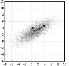
PCA of a 2D Gaussian centred at \((1, 3)\), with a standard deviation of 3 roughly along the direction \((0.866, 0.5)\) and of 1 in the orthogonal direction. The arrows are the eigenvectors of the covariance matrix, scaled by the square roots of their eigenvalues, with their tails at the mean. Adapted from: Principal component analysis
The least significant dimensions of the transformed data can now be discarded, reducing the number of features of the model. The number of eigenvectors kept in \(F\) dictates the amount of compression achieved. The first \(k\) components explain a fraction \(\sum_{i=1}^k \lambda_i / \sum_{i} \lambda_i\) of the variance of the data, a common criterion to choose \(k\).
To recover the original data (or an approximation, if \(F\) does not include all eigenvectors), the transformation is inverted, i.e. the transformed data is multiplied by the inverse of \(F^T\). The eigenvectors of the symmetric matrix \(C\) are orthonormal, so \(F^TF = I\). When \(F\) keeps all eigenvectors, it is square and orthogonal, so \(F^{-T} = F\) and:
\[D_c = F^{-T} D_n = F D_n\]When \(F\) keeps only \(k\) eigenvectors, \(F D_n\) is the projection of the data onto the first \(k\) principal components, the best approximation of \(D_c\) by \(k\) dimensions in the least-squares sense.
In practice, PCA is usually computed with the singular value decomposition of the centered data instead: if \(D_c^T = U \Sigma V^T\), the columns of \(V\) are the eigenvectors of \(C\), and its eigenvalues are \(\lambda_i = \sigma_i^2 / (n-1)\). This avoids computing \(C\), whose condition number is the square of that of \(D_c\), and is numerically more stable.
Kernel PCA
PCA only finds linear structure. Kernel PCA (Schölkopf et al., 1998) applies PCA in a high-dimensional feature space \(\phi(x)\), where non-linear structure of the input space may become linear. The kernel trick avoids computing \(\phi\), as the method only needs the dot products \(k(x_i, x_j) = \phi(x_i)^T \phi(x_j)\), given by a kernel function such as the Gaussian kernel \(k(x_i, x_j) = \exp \left( - \| x_i - x_j \|^2 / 2 \sigma^2 \right)\) or the polynomial kernel \(k(x_i, x_j) = (x_i^T x_j + c)^d\). The algorithm is:
- compute the \(n \times n\) kernel matrix \(K\), with \(K_{ij} = k(x_i, x_j)\);
- center the data in the feature space: \(\tilde{K} = K - 1_n K - K 1_n + 1_n K 1_n\), where \(1_n\) is the \(n \times n\) matrix with all entries equal to \(1/n\);
- compute the eigenvalues \(\lambda_m\) and eigenvectors \(\alpha^{(m)}\) of \(\tilde{K}\), and scale each eigenvector so that \(\lambda_m \, \alpha^{(m)T} \alpha^{(m)} = 1\), which gives the corresponding direction in the feature space a unit norm;
- the \(m\)-th principal component of a data point \(x_j\) is \(\sum_{i=1}^n \alpha_i^{(m)} \tilde{K}_{ij}\), i.e. the \(j\)-th entry of \(\tilde{K} \alpha^{(m)} = \lambda_m \alpha^{(m)}\).
The eigendecomposition of an \(n \times n\) matrix limits kernel PCA to datasets of moderate size, and mapping a point back to the input space (the pre-image problem) is only approximate. For the sake of comparison, the cost of PCA grows only linearly with the number of data points, as the size of its covariance matrix depends only on the number of features.
Independent Component Analysis
This section was largely inspired by the lecture notes of Tatsuya Yokota (Tokyo Institute of Technology, 2012).
A related topic is Independent Component Analysis (ICA), a method for blind source separation: it separates a multidimensional signal into additive subcomponents, under the assumptions that:
- the source signals \(s_1\), …, \(s_n\) are statistically independent, i.e. \(p(s_1, s_2, ..., s_n) = p(s_1)\,\,p(s_2) \,\, ... \,\, p(s_n)\);
- the sources are not Gaussian (at most one of them may be), otherwise ICA is impossible.
ICA builds on the Central Limit Theorem, which states that the distribution of the sum of \(N\) independent random variables approaches a Gaussian as \(N \rightarrow \infty\). As an example, the throw of a die has a uniform distribution from 1 to 6, but the distribution of the sum of several throws is better approximated by a Gaussian as the number of throws increases. A mixture of independent signals is thus more Gaussian than the signals themselves, and the most non-Gaussian directions recover the independent signals. In short, non-Gaussianity is independence.
A famous example is the cocktail party problem. A guest hears observed signals \(x\) that are mixtures of the original signals \(s\), as in:
\[\begin{align*} x_1(t) = a_{11}s_1(t) + a_{12}s_2(t) + a_{13}s_3(t)\\ x_2(t) = a_{21}s_1(t) + a_{22}s_2(t) + a_{23}s_3(t)\\ x_3(t) = a_{31}s_1(t) + a_{32}s_2(t) + a_{33}s_3(t) \end{align*}\]Assume that \(s_1\), \(s_2\) and \(s_3\) are statistically independent. The goal of ICA is to estimate the independent components \(s(t)\) from \(x(t)\), with
\[x(t) = As(t)\]where \(A\) is an invertible mixing matrix. Thus, the problem can be written as \(s(t) = Bx(t)\), where \(B = A^{-1}\). It is only necessary to estimate \(B\) so that the \(s_i\) are independent.
Signals \(z\) are white if they satisfy \(E [z] = 0\) and \(E [ z z^T ] = I\). Whitening is a useful pre-processing step for ICA. The whitened signals are \(z (t) = V x(t)\), where \(x\) is centered and \(V\) is the whitening matrix (e.g. \(V = \Lambda^{-1/2} F^T\), with the eigenvalues \(\Lambda\) and the eigenvectors \(F\) of the covariance matrix of \(x\), as in PCA). The model becomes:
\[s(t) = U z (t) = U V x (t) = B x (t)\]where \(U\) is an orthogonal matrix. Whitening simplifies ICA, as it is then only necessary to estimate \(U\): the whitened signals are already uncorrelated, like the principal components of PCA, and \(U\) is the rotation that makes them independent. An illustration of the source, observed and whitened data is displayed below, where the mixing turns the square of the sources into a parallelogram, and whitening turns it back into a square, rotated:
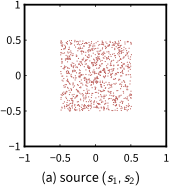
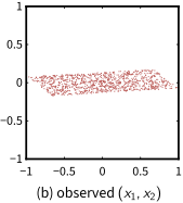
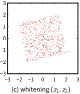
Independent component analysis of two mixed signals: (a) the sources \(s_1\), \(s_2\), independent and uniformly distributed; (b) the observed signals \(x_1\), \(x_2\), mixed as \(x = As\); (c) the whitened signals \(z_1\), \(z_2\), \(z = Vx\), with zero mean and identity covariance, from which only the orthogonal matrix \(U\) remains to be found. Adapted from: T. Yokota, Independent Component Analysis for Blind Source Separation, Tokyo Institute of Technology, 2012
Non-Gaussianity is a measure of independence. Kurtosis is a measure of non-Gaussianity, defined for a variable \(y\) of zero mean by:
\[\mathrm{kurt}(y) = E [y^4] - 3 (E[y^2])^2.\]It is zero for a Gaussian. Assume that \(y\) is white, i.e. \(E[y]=0\) and \(E[y^2]=1\), thus
\[\mathrm{kurt}(y) = E[y^4]-3.\]Each row \(b^T\) of \(B\) recovers one source, \(s_i = b^T x\). The ICA problem is solved with
\[\hat{b} = \arg\max_b | \mathrm{kurt}(b^T x(t)) |\]where \(b^T x(t)\) is constrained to unit variance. On the whitened data, \(b^T x(t) = w^T z(t)\), where \(w^T = b^T V^{-1}\) is a row of \(U\), and the unit-variance constraint becomes \(w^T w=1\). The absolute value of the kurtosis \(\mid \mathrm{kurt}(w^Tz) \mid\) is then maximized, subject to \(w^T w=1\). Its gradient is:
\[\begin{align*} \frac{\partial \vert \mathrm{kurt}(w^T z) \vert}{\partial w} & = \frac{\partial}{\partial w} \left\vert E[(w^T z)^4] - 3 (E[(w^T z)^2])^2 \right\vert \\ & = \frac{\partial}{\partial w} \left\vert E[(w^T z)^4] - 3 (\| w \|^2)^2 \right\vert \quad \text{(because } E[z z^T] = I) \\ & = 4 \, \text{sign}[\mathrm{kurt}(w^T z)] \left( E[z (w^T z)^3] - 3 w \| w \|^2 \right) \end{align*}\]The problem can now be solved by gradient ascent (with \(\| w \| = 1\)):
- \(\Delta w \propto \text{sign} [ \mathrm{kurt}(w^T z)] \, ( E [ z(w^T z)^3 ] - 3w )\);
- \(w \leftarrow w + \Delta w\), followed by the normalization \(w \leftarrow w / \| w \|\).
Or, because the algorithm converges when \(w \propto \Delta w\), and \(w\) and \(-w\) are equivalent, with the fixed-point iteration of FastICA (Hyvärinen and Oja, 1997):
- \(w \leftarrow E [ z ( w^T z)^3 ] - 3w\), followed by \(w \leftarrow w / \| w \|\).
Unlike gradient ascent, FastICA has no learning rate to tune, and its convergence is cubic, so it is usually much faster. The other components are found in the same way, keeping each new \(w\) orthogonal to the previous ones, as the rows of \(U\) are orthonormal.
As a final remark, kurtosis is very sensitive to outliers, because it is a fourth-order function. A more robust alternative is the negentropy. It is omitted here for brevity, but the details are in the original lecture notes.
Competitive Learning and k-means
Not to be confused with the k-nearest neighbours algorithm (KNN).
Competitive learning underlies the self-organization of the brain. In practice, neural network wiring is adaptive, not fixed, and competition drives wiring across all brain systems (motor cortex, neocortex, etc.). A common technique for data reduction from competitive learning is prototype clustering, where the data points \(x_u\) are represented by a smaller set of prototypes \(w_k\) that represent clusters of points. The general rule is that a new point \(x\) belongs to the closest prototype \(k\), i.e.
\[\| w_k - x \| \leq \| w_i - x \| \text{, for all } i\]This kind of partitioning underlies problems such as the Voronoi diagram for spatial data partitioning. A 2D example follows, where the points of each region (colored cells) belong to its prototype (black points):
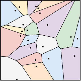
The Voronoi diagram of 20 prototypes (black dots) in 2D: each colored cell holds the points closer to its prototype than to any other, in Euclidean distance. Adapted from: Voronoi diagram
Such methods can be applied to e.g. image compression, where one may reduce every RGB pixel in the range \([0, 255]^3\) to the closest color of a smaller set. The reconstruction (squared) error is the sum of the errors of all data points over all clusters \(C_i\):
\[E = \sum_{i=1}^{k} \sum_{u \in C_i} \| w_i - x_u \|^2\]k-means clustering is an iterative method for prototype clustering. Its objective is to find the partition of the data points into \(k\) clusters \(C_1, ..., C_k\) that minimizes the error above:
\[\arg\min_{C_1, ..., C_k} \sum_{i=1}^{k} \sum_{x \in C_i} \| x - w_i \|^2\]where \(w_i\) is the mean of the points in \(C_i\). The algorithm iterates over 2 steps:
- assignment step: assign each observation to the closest mean, based on e.g. the Euclidean distance;
- update step: compute the new means as the centroids of the observations in each new cluster: \(w_i^{(t+1)} = \frac{1}{\mid C^{(t)}_i \mid} \sum_{x_j \in C_i^{(t)}} x_j\)
The algorithm converges when the assignments no longer change, and the means are then the centers of mass of their clusters. With the update \(\Delta w_i = \eta \sum_{u \in C_i} (x_u - w_i)\) over the \(N\) points of cluster \(C_i\), convergence means \(\Delta w_i = 0\), so it must hold that:
\[\eta \sum_{u \in C_i} (x_u - w_i) = 0 \rightarrow \sum_{u \in C_i} x_u - N w_i =0 \rightarrow w_i = \frac{1}{N} \sum_{u \in C_i} x_u\]which is the definition of the center of mass of cluster \(i\). The error decreases at every step and there is a finite number of partitions, so k-means always converges, but possibly to a local minimum. So it is usually run several times from different initial means, e.g. picked far from each other with k-means++. An illustration of the algorithm follows:
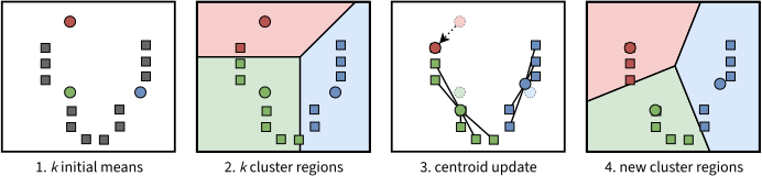
1. \(k = 3\) initial means (colored circles) are chosen at random within the data domain. 2. Assignment step: each point joins the cluster of the closest mean; the colored regions are the Voronoi cells of the means. 3. Update step: each mean moves to the centroid of its cluster (dashed circles: the previous means; lines: the points of each cluster). 4. Assignment step with the new means and their Voronoi cells: two points move from the green to the red cluster. The two steps repeat until the assignments no longer change. Adapted from: k-means clustering
In a 2D space, one can imagine a 3-cluster run as:

Iterations of k-means with \(k = 3\) on 2D data, with the Voronoi borders of the current means, until the assignments no longer change. Source: k-means clustering
The update rule above is a batch learning rule, as it updates the weights based on a set (batch) of inputs. The converse rule is the online update rule, which updates the weights of the winning prototype \(i\) at the introduction of every new input \(x_u\):
\[\Delta w_i = \eta (x_u - w_i)\]which is Oja’s Hebbian learning rule for a winner-take-all neuron, i.e. with an output \(y_i = 1\) for the winner and \(0\) for all other neurons.
K-means has 2 main problems:
- it forces the clusters to be spherical, while it is sometimes desirable to have elliptical clusters;
- each element can only belong to one cluster, which may not always be a good choice.
Both problems can be fixed with Gaussian mixture models. A mixture model is a mixture of distributions (in this case, Gaussians) that represents the probability distribution of the observations in the overall population.
Gaussian Mixture Models and Expectation-Maximization
A Gaussian mixture model (GMM) describes the data as drawn from \(K\) Gaussians: each data point picks a component \(k\) with probability \(\pi_k\), and is then drawn from the Gaussian \(\mathcal{N}(\mu_k, \Sigma_k)\), so that:
\[p(x) = \sum_{k=1}^K \pi_k \, \mathcal{N}(x \mid \mu_k, \Sigma_k), \text{ with } \sum_{k=1}^K \pi_k = 1.\]The covariance matrices \(\Sigma_k\) give each cluster an elliptical shape, and each point belongs to every cluster with some probability. The parameters are learned by maximizing the log-likelihood \(\sum_{n=1}^N \log p(x_n)\) of the \(N\) data points, with the Expectation-Maximization (EM) algorithm, which alternates two steps, like k-means:
- E-step: compute the responsibility of each component \(k\) for each point \(x_n\), i.e. the posterior probability that \(x_n\) was drawn from it:
- M-step: update the parameters, using the responsibilities as weights, with \(N_k = \sum_{n} \gamma_{nk}\):
Each iteration never decreases the log-likelihood, and the algorithm converges to a local maximum, so, as with k-means, it is usually run from several initializations, or initialized with the result of k-means. In fact, k-means is a limit case of EM: for a GMM whose components share the covariance \(\sigma^2 I\), the responsibilities become hard assignments to the closest mean as \(\sigma \rightarrow 0\). The number of components \(K\) can be chosen with a model selection criterion, such as the Bayesian information criterion. In practice, k-means is cheaper per iteration and is preferred for large datasets with compact clusters, while a GMM suits elliptical or overlapping clusters.
Hierarchical Clustering
Hierarchical clustering builds a tree of clusters (a dendrogram) instead of a single partition. Its common agglomerative (bottom-up) variant starts with one cluster per data point, and repeatedly merges the two closest clusters, until a single cluster remains. The distance between two clusters \(A\) and \(B\) is given by the linkage criterion:
- single linkage: the distance between their closest points, \(\min_{a \in A, b \in B} d(a,b)\). It finds elongated clusters, but can chain distinct clusters together through a few close points;
- complete linkage: the distance between their farthest points, \(\max_{a \in A, b \in B} d(a,b)\), which favours compact clusters;
- average linkage: the average distance between all pairs of points, \(\frac{1}{\mid A \mid \mid B \mid} \sum_{a \in A} \sum_{b \in B} d(a,b)\);
- Ward’s linkage: the increase of the k-means error (the sum of squared distances to the cluster means) caused by merging \(A\) and \(B\), which is \(\frac{\mid A \mid \mid B \mid}{\mid A \mid + \mid B \mid} \| \mu_A - \mu_B \|^2\) for cluster means \(\mu_A\) and \(\mu_B\).
Cutting the dendrogram at a given height yields a partition, so the number of clusters can be chosen after the fact, by looking at the tree. The divisive (top-down) variant does the opposite: it starts with all points in one cluster, and splits clusters recursively. Agglomerative clustering needs the \(n \times n\) matrix of pairwise distances, and runs in \(O(n^2)\) to \(O(n^3)\) time depending on the linkage and the implementation, so it suits small to medium datasets.
DBSCAN
DBSCAN (Density-Based Spatial Clustering of Applications with Noise, Ester et al., 1996) defines clusters as dense regions separated by sparse ones. It takes two parameters, a radius \(\varepsilon\) and a minimum number of points \(m\), and labels each point as:
- a core point, if at least \(m\) points (itself included) lie within distance \(\varepsilon\) of it;
- a border point, if it is not a core point but lies within distance \(\varepsilon\) of a core point;
- noise, otherwise.
Two core points within distance \(\varepsilon\) of each other belong to the same cluster, so each cluster is a connected group of core points, plus the border points around them. Unlike k-means, DBSCAN does not need the number of clusters, finds clusters of arbitrary shapes, and labels outliers as noise. On the other hand, a single radius \(\varepsilon\) cannot capture clusters of very different densities, a limitation addressed by its extensions OPTICS and HDBSCAN. In low dimensions, a spatial index finds the neighbours of each point without computing all pairwise distances.
Spectral Clustering
Spectral clustering treats clustering as a graph partitioning problem. It builds a graph of the data points, with a similarity \(W_{ij}\) for each pair of points, e.g. \(W_{ij} = \exp ( - \| x_i - x_j \|^2 / 2\sigma^2 )\) between each point and its nearest neighbours and \(0\) otherwise, and looks for clusters connected by edges of little weight. With the degree matrix \(D\), a diagonal matrix with \(D_{ii} = \sum_j W_{ij}\), the graph Laplacian is \(L = D - W\), and for any vector \(f\):
\[f^T L f = \frac{1}{2} \sum_{i,j} W_{ij} (f_i - f_j)^2\]So \(f^T L f\) is small when \(f\) takes similar values on strongly connected points, and the eigenvectors of \(L\) with the smallest eigenvalues vary little within clusters. In particular, the multiplicity of the eigenvalue \(0\) is the number of connected components of the graph. The algorithm is:
- compute the eigenvectors \(u_1, ..., u_k\) of the \(k\) smallest eigenvalues of \(L\), or of the normalized Laplacian \(L_{sym} = I - D^{-1/2} W D^{-1/2}\);
- stack them as the columns of an \(n \times k\) matrix \(H\), and take its \(i\)-th row as the new \(k\)-dimensional representation of point \(x_i\) (with \(L_{sym}\), after normalizing each row to unit length);
- cluster the rows of \(H\) with k-means.
This is a relaxation of the NP-hard problem of finding the ratio cut (with \(L\)) or the normalized cut (with \(L_{sym}\)) of the graph. Spectral clustering separates non-convex clusters (e.g. two concentric rings) that k-means cannot, at the cost of an eigendecomposition of an \(n \times n\) (sparse) matrix.
For more details, A Tutorial on Spectral Clustering (von Luxburg, 2007) derives these algorithms from graph cuts, random walks and perturbation theory, and discusses which graph Laplacian to use.
Self-Organizing Maps and Kohonen Maps
A self-organizing map (SOM) is an unsupervised artificial neural network, typically a 2D grid of neurons, that represents a discretization of the input space (or of the training set). It was introduced by Teuvo Kohonen in the paper Self-organized formation of topologically correct feature maps (1982), hence its other name, the Kohonen map. Its main purpose is to represent the training data by localized regions (neurons) that represent agglomerates of inputs, with neighbouring neurons of the grid representing nearby regions of the input space. The following picture illustrates Kohonen’s model (top) and one step of its learning algorithm (bottom):
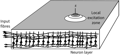
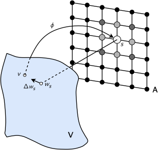
Top: the neuron layer of Kohonen’s model. The input fibres running horizontally carry the input signal (the stimulus) and excite the neurons of the layer through synaptic connections. Lateral interactions between the neurons confine the response to a spatially bounded local excitation zone. The layer acts as a topographic feature map if the position \(s\) of the excitation zone varies continuously with the stimulus features of interest. Bottom: the adaptation step. The input \(v\) in the input space \(V\) selects the winner neuron \(s\) in the lattice of neurons \(A\) (\(\phi\) is the map from \(V\) to \(A\)). The winner and its neighbours shift their weight vectors towards \(v\), by an amount that decreases with the distance from \(s\), shown by the sizes and gray levels of the neurons. Only the shift \(\Delta w_s\) of the winner’s weights \(w_s\) is drawn. In the algorithm below, \(v\) is the input \(x_u\) and \(s\) is the winner \(j^*\). Adapted from: Neural Computation and Self-Organizing Maps, H. Ritter, T. Martinetz and K. Schulten, 1992, Figures 4.1 and 4.2
The algorithm is the following:
- neurons are randomly placed in the multidimensional space;
- at every iteration, choose an input \(x_u\);
- determine which neuron \(j^*\) is the winner (or best matching unit, BMU), i.e. the closest in space:
- update the weights of the winner and of its neighbours, by pulling them closer to the input vector:
where \(h(j, j^*)\) is the neighbourhood function, which decreases with the distance between neurons \(j\) and \(j^*\) in the grid (e.g. a Gaussian). If \(h\) is \(1\) for the winner and \(0\) for all other neurons, the update above is the online update rule of k-means. It is also common to decrease \(\eta\) and the width of \(h\) as the iterations progress;
- repeat until stabilization: either when reaching the maximum number of iterations, or when the change in weights falls below a given threshold.
Very nice videos demonstrating an iterative execution of the Kohonen map can be found in this link and this link.
A good example is the recognition of handwritten digits from the MNIST database. Each digit is a 28x28 (=784) pixel array, represented as a data point in a 784-dimensional space. Each pixel is monochromatic, so each dimension takes values between 0 and 255.
The task is, given a database of 5000 handwritten digits, to find the 6x6 SOM that best represents 4 of the digits from 0 to 9. This example studies how the neighbourhood width and the learning rate affect the performance of the Kohonen map.
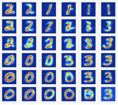
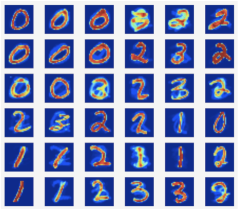
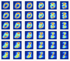
The input dataset and the python implementation are available in kohonen_mnist.zip. The goal is to fine-tune the neighbourhood width and the learning rate \(\eta\). A good solution gives a visual perception of the digits being identified (in this case 0, 1, 2 and 3), as the weights of each neuron form a 28x28 image. Three possible outputs are displayed in the pictures below:
- left: a nicely tuned SOM, where each quadrant of neurons represents a digit;
- center: a SOM with a high learning rate. The large step size makes neurons step over long distances during training, leading to a mixing of digits on nearby neurons, and possibly a tangled SOM;
- right: a SOM with a large neighbourhood width. The large width causes all neurons to behave almost synchronously, due to the very wide range of the update function. This leads to very similar outputs per neuron.
More examples can be found in the Wikipedia entry for self-organizing maps.
t-SNE and UMAP
PCA preserves the global, linear structure of the data, which is often not what one wants to see when visualizing high-dimensional data in 2D or 3D. Neighbour embedding methods instead place similar points close together, preserving local neighbourhoods.
t-SNE (t-distributed Stochastic Neighbor Embedding, van der Maaten and Hinton, 2008) turns distances into probabilities. In the input space, the similarity of point \(x_j\) to point \(x_i\) is:
\[p_{j \mid i} = \frac{\exp \left( - \| x_i - x_j \|^2 / 2 \sigma_i^2 \right)}{\sum_{k \neq i} \exp \left( - \| x_i - x_k \|^2 / 2 \sigma_i^2 \right)}\]where each \(\sigma_i\) is set so that the distribution \(p_{\cdot \mid i}\) has a given perplexity (roughly, the number of effective neighbours, typically 5 to 50), and the symmetric similarity of the pair is \(p_{ij} = (p_{j \mid i} + p_{i \mid j}) / 2n\). In the low-dimensional embedding \(y_1, ..., y_n\), similarities follow a Student t-distribution with one degree of freedom:
\[q_{ij} = \frac{\left(1 + \| y_i - y_j \|^2 \right)^{-1}}{\sum_{k \neq l} \left( 1 + \| y_k - y_l \|^2 \right)^{-1}}\]and the embedding minimizes the Kullback-Leibler divergence \(KL(P \| Q) = \sum_{i \neq j} p_{ij} \log (p_{ij} / q_{ij})\) by gradient descent, with:
\[\frac{\partial KL}{\partial y_i} = 4 \sum_{j} (p_{ij} - q_{ij}) (y_i - y_j) \left( 1 + \| y_i - y_j \|^2 \right)^{-1}\]The heavy tails of the t-distribution let moderately distant points move far apart in the embedding. This avoids the crowding problem that a Gaussian would have in low dimensions, and produces well-separated clusters. Two caveats: the sizes of the clusters and the distances between them in a t-SNE plot carry little meaning, and the result depends on the perplexity and the random initialization. Each iteration costs \(O(n^2)\), or \(O(n \log n)\) with the Barnes-Hut approximation.
UMAP (Uniform Manifold Approximation and Projection, McInnes et al., 2018) follows the same idea with a different construction. It builds a weighted graph of the \(k\) nearest neighbours of each point, with weights:
\[v_{j \mid i} = \exp \left( - \frac{d(x_i, x_j) - \rho_i}{\sigma_i} \right)\]where \(\rho_i\) is the distance from \(x_i\) to its nearest neighbour, and \(\sigma_i\) is set so that \(\sum_j v_{j \mid i} = \log_2 k\). The weights are made symmetric as \(v_{ij} = v_{j \mid i} + v_{i \mid j} - v_{j \mid i} \, v_{i \mid j}\). In the embedding, the similarities are \(w_{ij} = \left( 1 + a \| y_i - y_j \|^{2b} \right)^{-1}\), with \(a\) and \(b\) set by the minimum distance between embedded points, and the embedding minimizes the cross-entropy between the two graphs:
\[\sum_{i \neq j} v_{ij} \log \frac{v_{ij}}{w_{ij}} + (1 - v_{ij}) \log \frac{1 - v_{ij}}{1 - w_{ij}}\]with stochastic gradient descent and negative sampling. The second term pushes apart the points that are not neighbours, and UMAP tends to preserve more of the global structure than t-SNE, although mostly due to its spectral initialization (Kobak and Linderman, 2021). It is also faster, scales to millions of points and can embed new points, so it is used as a general dimensionality reduction method too, and not only for visualization.
Autoencoders and Self-Supervised Learning
An autoencoder is a neural network trained to reproduce its input. An encoder \(f\) maps the input \(x\) to a lower-dimensional code \(z = f(x)\), and a decoder \(g\) maps the code back to a reconstruction \(\hat{x} = g(z)\). Both are trained together to minimize the reconstruction error, e.g.:
\[\min_{f, g} \sum_{n} \| x_n - g(f(x_n)) \|^2\]The narrow code (the bottleneck) forces the network to keep only the most informative features of the data. A linear autoencoder trained with the squared error learns the same subspace as PCA (although not necessarily the principal components themselves), so an autoencoder with non-linear activations is a non-linear generalization of PCA. Common variants are:
- sparse autoencoders, that add a penalty on the code activations (e.g. their L1 norm), so that each input activates only a few features, even when the code is larger than the input;
- denoising autoencoders, that reconstruct the clean input \(x\) from a corrupted version \(\tilde{x}\) (e.g. with added noise or masked entries), which forces them to learn the structure of the data instead of the identity function;
- variational autoencoders, that learn a distribution over the codes, which turns the decoder into a generative model.
Denoising autoencoders are an early example of self-supervised learning: the training targets come from the data itself, by hiding part of the input and predicting it. This is how most large models are pretrained today: language models predict the next token of a text, BERT (Devlin et al., 2018) predicts masked words, and masked autoencoders (He et al., 2021) reconstruct masked patches of images. Contrastive learning is another self-supervised approach: methods like SimCLR (Chen et al., 2020) create two augmented views of each image. An encoder is then trained so that the embeddings \(z_i\) and \(z_j\) of two views of the same image are close, and far from the embeddings of the other images in the batch, with the loss:
\[\ell_{i,j} = - \log \frac{\exp \left( \text{sim}(z_i, z_j) / \tau \right)}{\sum_{k \neq i} \exp \left( \text{sim}(z_i, z_k) / \tau \right)}\]where \(\text{sim}\) is the cosine similarity and \(\tau\) is a temperature. The representations learned this way can then be used for clustering or retrieval, or fine-tuned on a supervised task with few labels.
The Curse of Dimensionality
As a final remark, distance-based methods struggle with high-dimensional data, in particular with Euclidean distances. This is due to a phenomenon called the curse of dimensionality: as the number of dimensions increases, the distances between any two points become similar, which makes the distance metric almost irrelevant. For example, for points with independent and identically distributed coordinates, the relative difference between the distances from a point to its farthest and nearest neighbours, \((d_{max} - d_{min}) / d_{min}\), tends to 0 as the number of dimensions grows (Beyer et al., 1999).
The soundness of the claim is not detailed here, but this blog post covers the curse of dimensionality in more detail. This phenomenon is one more reason to reduce the dimensionality of the data, e.g. with PCA, before clustering it.
To find more about the topic, the book Pattern Recognition and Machine Learning by Christopher Bishop covers k-means, Gaussian mixtures and the EM algorithm (chapter 9), and PCA, kernel PCA, ICA and autoencoders (chapter 12).