Diffusion models: from DDPMs to DiTs
Despite dating back to 2015, diffusion models (DMs) only gained momentum after the paper Denoising Diffusion Probabilistic Models. Just like GANs or VAEs, diffusion models are generative models that learn to convert noise from a distribution into a data sample - the “denoising” process. A diffusion model is made of two Markov chains: a forward process that gradually adds noise to the data, and a learnable reverse process that performs the denoising. The transitions of the reverse chain are learned with variational inference. Once the model is trained, a sampling algorithm can generate new data from pure noise.
In this post, we will look at the mathematical background behind diffusion models, and implement a U-Net- and a Transformer-based diffusion model. We will then look into high dimensionality inputs such as videos, and how video diffusion models handle them with compressed latent representations and spatio-temporal attention.

A diffusion model is a \(T\)-step Markov chain, characterized by a forward process \(q\) and a trainable reverse process \(p_\theta\). Source: Denoising Diffusion Probabilistic Models.
Let’s look at those processes in detail. Credit: formulation and U-Net implementation inspired by the paper Denoising Diffusion Probabilistic Models, Hugging Face’s post The Annotated Diffusion Model and Lilian Weng’s post Lil’Log: what are diffusion models. The learned variance and the noise schedule for a smaller number of steps follow Improved Denoising Diffusion Probabilistic Models and its official implementation. The full code is available in diffusion.py and dit.py.
Forward Process
The forward diffusion process \(q\) is a Markov chain that performs \(T\) steps, where each step gradually adds Gaussian noise to the previous step, according to a variance \(\beta_t \in (0,1)\) for all \(T\) timesteps, typically with \(0 \lt \beta_1 \lt \beta_2 \lt ... \lt \beta_T < 1\). \(\beta_t\) can be learned or (in this case) fixed as a hyper-parameter. We start with our data as \(\mathbf{x}_0\) for \(t=0\) and gradually sample and add Gaussian noise at each step, producing noisy samples \(\mathbf{x}_1, ..., \mathbf{x}_T\). The forward process \(q\) is then represented as (Eq. 2 in paper):
\[q(\mathbf{x}_t \vert \mathbf{x}_{t-1}) = \mathcal{N}(\mathbf{x}_t; \sqrt{1 - \beta_t} \mathbf{x}_{t-1}, \beta_t\mathbf{I}) \quad\]ie each new sample \(\mathbf{x}_t\) is drawn from a Gaussian distribution with mean \(\mu_t = \sqrt{1-\beta_t} \mathbf{x}_{t-1}\) and variance \(\sigma^2_t = \beta_t\). When \(T \rightarrow \infty\), we end up with an isotropic Gaussian distribution at \(t=T\). An isotropic Gaussian is one where the covariance matrix \(\Sigma\) is represented by \(\Sigma=\sigma^2\mathbf{I}\), where \(\sigma^2 \in \mathbb{R}\) is the variance constant and \(\mathbf{I}\) is the identity matrix.
This is equivalent to sampling \(\epsilon \sim \mathcal{N}(0, \mathbf{I})\) and then setting \(\mathbf{x}_t = \sqrt{1-\beta_t} \mathbf{x}_{t-1} + \sqrt{\beta_t}\epsilon\).
Another property in the forward process, demonstrated by Sohl-Dickstein et al., is that because the sum of independent Gaussian random variables is also a Gaussian random variable, we can sample \(\mathbf{x}_t\) at any time \(t\), conditioned directly on \(\mathbf{x}_0\), instead of conditioned on \(\mathbf{x}_{t-1}\) (ie iteratively). So we have that (Eq. 4 in paper):
\[q (\mathbf{x}_t \mid \mathbf{x}_0) = \mathcal{N} (\mathbf{x}_t ; \sqrt{\bar{\alpha}_t} \mathbf{x}_0, (1-\bar{\alpha}_t) \mathbf{I})\]where \(\alpha_t = 1 - \beta_t\) and \(\bar{\alpha}_t = \prod_{s=1}^t \alpha_s\).
We can start implementing our diffusion algorithm by defining the hyper-parameters \(\beta_t\) and \(\alpha_t\) and, for convenience, an additional \(\bar{\alpha}_t = \prod_{s=1}^t \alpha_s\). There are many \(\beta_t\) variance schedulers, but for simplicity, we will implement a linear scheduler \(\beta_t\). Note that Eq. 4 also tells us how much of the signal \(\mathbf{x}_0\) is left at the last step: \(\mathbf{x}_T\) is close to pure noise \(\mathcal{N}(0, \mathbf{I})\) only if \(\bar{\alpha}_T \approx 0\). The paper uses \(T=1000\) steps and a \(\beta_t\) that increases linearly from \(\beta_1=10^{-4}\) to \(\beta_T=0.02\), leading to \(\sqrt{\bar{\alpha}_T} \approx 0.006\). To sample faster, we will use \(T=100\) steps instead. Keeping the same \(\beta_1\) and \(\beta_T\) would then lead to \(\sqrt{\bar{\alpha}_T} \approx 0.6\), ie \(\mathbf{x}_T\) would keep 60% of the amplitude of \(\mathbf{x}_0\), and sampling from pure noise would not match what the model saw during training. So, as in the official implementation of Improved DDPM, we scale both values by \(1000/T\), leading to \(\sqrt{\bar{\alpha}_T} \approx 0.005\):
    T = 100 # the paper uses T=1000
    β_1, β_T = 0.0001 * 1000 / T, 0.02 * 1000 / T # the paper's values, scaled by 1000/T
    # arrays are 0-indexed: index i holds the value of the paper's timestep t=i+1
    β = torch.linspace(β_1, β_T, T, device=device)
    α = 1. - β
    α_cumprod = torch.cumprod(α, axis=0)
Now we define the Sohl-Dickstein’s forward process \(q (\mathbf{x}_t \mid \mathbf{x}_0)\) as:
    @torch.no_grad()
    def q_sample(x0, t, noise=None):
        # note that in Eq 4, it samples from a non-standard gaussian distribution, but here we implement it
        # by sampling from the standard normal (0,1) and shifting and scaling it later, which is equivalent
        # Detailed in the paragraph between equations 8 and 9, and applied in algorithm 1, step 4, the epsilon.
        if noise is None:
            noise = torch.randn_like(x0) # samples from N(0,1)
        sqrt_α_cumprod = torch.sqrt(α_cumprod)
        sqrt_α_cumprod_t = sqrt_α_cumprod[t][:, None, None, None]
        sqrt_1_minus_α_cumprod = torch.sqrt(1. - α_cumprod)
        sqrt_1_minus_α_cumprod_t = sqrt_1_minus_α_cumprod[t][:, None, None, None]
        return sqrt_α_cumprod_t * x0 + sqrt_1_minus_α_cumprod_t * noise
The other property is that the forward process posterior is tractable when conditioned on \(\mathbf{x}_0\), so it can be written as:
\[q(\mathbf{x}_{t-1} \mid \mathbf{x}_t, \mathbf{x}_0 ) = \mathcal{N} (\mathbf{x}_{t-1} ; \tilde{\mu}_t (\mathbf{x}_t, \mathbf{x}_0), \, \tilde{\beta}_t \mathbf{I})\]where \(\tilde{\beta}_t\) is the posterior variance, a constant that depends only on the noise schedule, computed as (Eq. 7 in paper):
\[\tilde{\beta}_t = \frac{1-\bar{\alpha}_{t-1}}{1-\bar{\alpha}_t} \beta_t\]and that can be coded as below. We also compute its logarithm, that we will use later to learn the variance in the DiT section. As \(\tilde{\beta}_t\) is zero at the first timestep, its log is clipped to the value of the second timestep, as in the official implementation:
    # posterior variance, and its log clipped at index 0 (where posterior_β is 0)
    α_cumprod_prev = F.pad(α_cumprod[:-1], (1, 0), value=1.0)
    posterior_β = β * (1. - α_cumprod_prev) / (1. - α_cumprod) # Eq 7
    posterior_log_β = torch.log(torch.cat([posterior_β[1:2], posterior_β[1:]]))
and \(\tilde{\mu}_t\) is the posterior mean for the timestep \(t\) (Eq. 7):
\[\tilde{\mu}_t(\mathbf{x}_t, \mathbf{x}_0) = \frac{\sqrt{\bar{\alpha}_{t-1}} \beta_t }{1-\bar{\alpha}_t} \mathbf{x}_0 + \frac{\sqrt{\alpha_t}(1-\bar{\alpha}_{t-1})}{1-\bar{\alpha}_t} \mathbf{x}_t\]coded as the function:
    @torch.no_grad()
    def posterior_μ(x_0, x_t, t):
        """ return posterior mean at step t, Equation 7 """
        α_t = α[t][:, None, None, None]
        β_t = β[t][:, None, None, None]
        α_cumprod_t = α_cumprod[t][:, None, None, None]
        α_cumprod_prev_t = α_cumprod_prev[t][:, None, None, None]
        coef1 =  β_t * torch.sqrt(α_cumprod_prev_t) / (1.0 - α_cumprod_t)
        coef2 = (1.0 - α_cumprod_prev_t) * torch.sqrt(α_t) / (1.0 - α_cumprod_t)
        return coef1 * x_0 + coef2 * x_t
Reverse process
The reverse process is a Markov chain \(p_\theta(\mathbf{x}_{0:T})\) with learned Gaussian transitions starting at \(p(\mathbf{x}_T) = \mathcal{N} (\mathbf{x}_T ; 0, \mathbf{I})\), and:
\[p_\theta(\mathbf{x}_{t-1} \vert \mathbf{x}_t) = \mathcal{N}(\mathbf{x}_{t-1}; \boldsymbol{\mu}_\theta(\mathbf{x}_t, t), \boldsymbol{\Sigma}_\theta(\mathbf{x}_t, t) )\]We do not know the distribution of the true denoising step \(q(\mathbf{x}_{t-1} \mid \mathbf{x}_t)\), as it depends on the whole data distribution, so we approximate it with \(p_{\theta}\), parameterized by a neural network. We assume this distribution to be Gaussian, with a learnable mean \(\mu_\theta\) and covariance \(\Sigma_\theta\) (Eq. 1 in the paper). This is a good approximation when the \(\beta_t\) are small, as the reverse of a small Gaussian diffusion step is also (approximately) Gaussian.
In the original paper, the variance \(\Sigma_\theta (\mathbf{x}_t, t)\) is not learned, and it’s set as \(\Sigma_\theta(\mathbf{x}_t, t) = \sigma^2_t \mathbf{I}\) and \(\sigma^2_t = \beta_t\) or \(\sigma^2_t = \tilde{\beta}_t\) (similar results). Learning \(\Sigma_\theta\) was later explored by Improved Denoising Diffusion Probabilistic Models, and we will use it in the DiT section below.
In order to train \(p_\theta\), we can treat the combination of \(q\) and \(p_\theta\) as a variational auto-encoder, and maximize the evidence lower bound (ELBO) of the log-likelihood of the data \(\mathbf{x}_0\), or equivalently minimize the variational bound \(L\) on the negative log-likelihood (Eq. 3 in the paper):
\[\mathbb{E} \left[ - \log p_\theta(\mathbf{x}_0) \right] \le \mathbb{E}_q \left[ - \log \frac{p_\theta(\mathbf{x}_{0:T})}{q(\mathbf{x}_{1:T} \vert \mathbf{x}_0)} \right] = \mathbb{E}_q \left[ - \log p(\mathbf{x}_T) - \sum_{t \ge 1} \log \frac{p_\theta(\mathbf{x}_{t-1} \vert \mathbf{x}_t)}{q(\mathbf{x}_t \vert \mathbf{x}_{t-1})} \right] =: L\]Taking the log turns the products over timesteps into a sum of terms. Using the forward process posteriors \(q(\mathbf{x}_{t-1} \mid \mathbf{x}_t, \mathbf{x}_0)\) defined above, this bound can be rewritten as (Eq. 5 in the paper):
\[L = \mathbb{E}_q \bigg[ \underbrace{D_{KL}(q(\mathbf{x}_T \vert \mathbf{x}_0) \parallel p(\mathbf{x}_T))}_{L_T} + \sum_{t > 1} \underbrace{D_{KL}(q(\mathbf{x}_{t-1} \vert \mathbf{x}_t, \mathbf{x}_0) \parallel p_\theta(\mathbf{x}_{t-1} \vert \mathbf{x}_t))}_{L_{t-1}} \underbrace{- \log p_\theta(\mathbf{x}_0 \vert \mathbf{x}_1)}_{L_0} \bigg]\]where \(L_T\) has no learnable parameters (it’s a constant), \(L_0\) is the reconstruction term of the last denoising step, and each \(L_{t-1}\) is a KL divergence between 2 Gaussian distributions and therefore has a closed form.
Let’s look at the terms \(L_{t-1}\) first. With \(\Sigma_\theta = \sigma_t^2 \mathbf{I}\), the KL divergence between the posterior \(q(\mathbf{x}_{t-1} \mid \mathbf{x}_t, \mathbf{x}_0) = \mathcal{N}(\tilde{\mu}_t, \tilde{\beta}_t \mathbf{I})\) and \(p_\theta(\mathbf{x}_{t-1} \mid \mathbf{x}_t) = \mathcal{N}(\mu_\theta, \sigma_t^2 \mathbf{I})\) is (Eq. 8 in the paper):
\[L_{t-1} = \mathbb{E}_q \left[ \frac{1}{2 \sigma_t^2} \| \tilde{\mu}_t(\mathbf{x}_t, \mathbf{x}_0) - \mu_\theta(\mathbf{x}_t, t) \|^2 \right] + C\]where \(C\) is a constant that does not depend on \(\theta\). So the most straightforward parameterization is a model \(\mu_\theta\) that predicts the posterior mean \(\tilde{\mu}_t\). However, we can expand it further by reparameterizing Eq. 4 as \(\mathbf{x}_t(\mathbf{x}_0, \epsilon) = \sqrt{\bar{\alpha}_t} \mathbf{x}_0 + \sqrt{1-\bar{\alpha}_t} \epsilon\) for \(\epsilon \sim \mathcal{N}(0, \mathbf{I})\), ie \(\mathbf{x}_0 = \frac{1}{\sqrt{\bar{\alpha}_t}} \left( \mathbf{x}_t - \sqrt{1-\bar{\alpha}_t} \epsilon \right)\), and replacing \(\mathbf{x}_0\) in the posterior mean \(\tilde{\mu}_t\) of Eq. 7 (Eqs. 9 and 10 in the paper):
\[L_{t-1} - C = \mathbb{E}_{\mathbf{x}_0, \epsilon} \left[ \frac{1}{2 \sigma_t^2} \left\| \frac{1}{\sqrt{\alpha_t}} \left( \mathbf{x}_t(\mathbf{x}_0, \epsilon) - \frac{\beta_t}{\sqrt{1-\bar{\alpha}_t}} \epsilon \right) - \mu_\theta(\mathbf{x}_t(\mathbf{x}_0, \epsilon), t) \right\|^2 \right]\]So \(\mu_\theta\) must predict \(\frac{1}{\sqrt{\alpha_t}} \left( \mathbf{x}_t - \frac{\beta_t}{\sqrt{1-\bar{\alpha}_t}} \epsilon \right)\) given \(\mathbf{x}_t\). As \(\mathbf{x}_t\) is already an input of the model, the authors propose a parameterization (section 3.2) where the model learns the noise \(\epsilon_\theta(\mathbf{x}_t, t)\) for step \(t\) instead of the mean \(\boldsymbol{\mu}_\theta(\mathbf{x}_t, t)\). The mean can then be computed as (Eq. 11 in paper):
\[\mu_\theta(\mathbf{x}_t, t) = \frac{1}{\sqrt{\alpha_t}} \left( \mathbf{x}_t - \frac{\beta_t}{\sqrt{1-\bar{\alpha}_t}} \epsilon_\theta(\mathbf{x}_t, t) \right)\]where the model \(\epsilon_\theta(\mathbf{x}_t, t)\) takes as input the image \(\mathbf{x}_t\) sampled at the timestep \(t\), and also the timestep \(t\) that will be used to add the timestep embedding. This is then coded as:
    def eq11_μ_θ(x, ε_θ, t):
        # Equation 11: use model (noise predictor) to predict the mean
        β_t = β[t][:, None, None, None]
        one_over_sqrt_α = torch.sqrt(1.0 / α)
        one_over_sqrt_α_t = one_over_sqrt_α[t][:, None, None, None]
        sqrt_1_minus_α_cumprod = torch.sqrt(1. - α_cumprod)
        sqrt_1_minus_α_cumprod_t = sqrt_1_minus_α_cumprod[t][:, None, None, None]
        μ_θ = one_over_sqrt_α_t * (x - β_t * ε_θ  / sqrt_1_minus_α_cumprod_t)
        return μ_θ
Replacing \(\mu_\theta\) by Eq. 11 in the loss above, each term \(L_{t-1}\) becomes a weighted mean squared error between the sampled and the predicted noise (Eq. 12 in the paper):
\[L_{t-1} - C = \mathbb{E}_{\mathbf{x}_0, \epsilon} \left[ \frac{\beta_t^2}{2 \sigma_t^2 \alpha_t (1-\bar{\alpha}_t)} \| \epsilon - \epsilon_\theta(\sqrt{\bar{\alpha}_t} \mathbf{x}_0 + \sqrt{1-\bar{\alpha}_t} \epsilon, t) \|^2 \right]\]The authors note that this objective resembles denoising score matching over multiple noise levels, and that sampling with Eq. 11 resembles Langevin dynamics with \(\epsilon_\theta\) as a learned gradient of the data density.
Finally, the last term \(L_0\) uses a discrete decoder. Image pixels are integers in \(\{0, 1, ..., 255\}\) scaled linearly to \([-1, 1]\), so the likelihood of each pixel value is the probability mass of \(p_\theta\) in a bin of width \(2/255\) around it, where the first and last bins extend to infinity (Eq. 13 in the paper):
\[p_\theta(\mathbf{x}_0 \mid \mathbf{x}_1) = \prod_{i=1}^D \int_{\delta_-(x_0^i)}^{\delta_+(x_0^i)} \mathcal{N}(x; \mu_\theta^i(\mathbf{x}_1, 1), \sigma_1^2) \, dx \quad \text{with} \quad \delta_+(x) = \begin{cases} \infty & \text{if } x = 1 \\ x + \frac{1}{255} & \text{if } x < 1 \end{cases} \quad \text{and} \quad \delta_-(x) = \begin{cases} -\infty & \text{if } x = -1 \\ x - \frac{1}{255} & \text{if } x > -1 \end{cases}\]where \(D\) is the data dimensionality and \(i\) indexes one coordinate. Its negative log-likelihood, per pixel value and for a given distribution \(p_\theta\), can be coded as:
    def eq13_decoder_nll(x_0, p):
        """ Equation 13: negative log-likelihood of the discretized decoder p_θ(x_0|x_1), per pixel value """
        cdf_upper = p.cdf(x_0 + 1/255) # CDF at δ+(x_0), for x_0 < 1
        cdf_lower = p.cdf(x_0 - 1/255) # CDF at δ-(x_0), for x_0 > -1
        # the CDF at -∞ and +∞ is 0 and 1 (evaluating it at ±∞ would make the gradients NaN)
        prob = torch.where(x_0 < -0.999, cdf_upper, torch.where(x_0 > 0.999, 1 - cdf_lower, cdf_upper - cdf_lower))
        return -torch.log(prob.clamp(min=1e-12))
Sampling
Once the model is trained, to generate new images we must reverse the diffusion process (from time T to time 1):
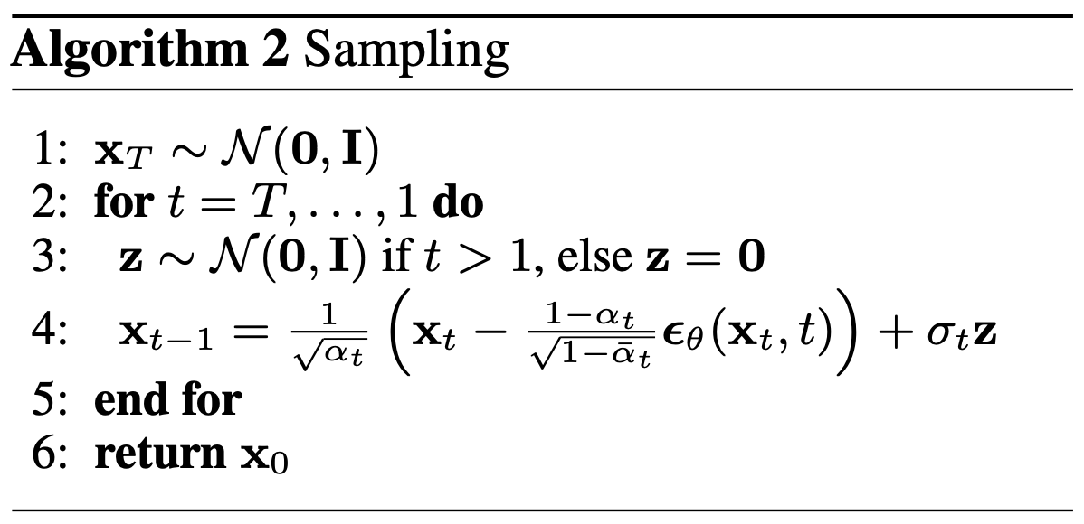
Step 4 samples \(\mathbf{x}_{t-1}\) by summing the predicted mean \(\mu_\theta(\mathbf{x}_t, t)\) with noise \(\mathbf{z}\) multiplied by the standard deviation \(\sigma_t\), where \(\sigma^2_t = \tilde{\beta}_t\) for the U-Net, and the learned variance \(\Sigma_\theta\) for the DiT (see the DiT section below). As in the paper, the model used for sampling is an Exponential Moving Average of the trained model weights (see the training section below):
    @torch.no_grad()
    def alg2_p_sampling(model, shape):
        img = torch.randn(shape, device=device) # step 1
        for t_index in reversed(range(0, T)): # step 2
            t = torch.full((shape[0],), t_index, device=device, dtype=torch.long)
            if model_name == 'UNet':
                ε_θ = model(img, t).sample # extract tensor from UNet2DOutput class
                σ2_t = posterior_β[t][:, None, None, None] # σ_t^2 = β̃_t
            else:
                ε_θ, v = model(img, t)
                σ2_t = learned_Σ_θ(v, t) # σ_t^2 = Σ_θ, learned
            img = eq11_μ_θ(img, ε_θ, t) # Eq. 11
            if t_index > 0: # step 3: z = 0 at the last step (paper's t=1)
                img += torch.sqrt(σ2_t) * torch.randn_like(img) # step 4
        return img
Training algorithm
We’ll train our model with the CIFAR10 dataset containing 32x32 RGB images across 10 classes. We’ll set our batch size to 48 images per batch (per GPU):
    # load dataset from the hub
    dataset = load_dataset("uoft-cs/cifar10", split='train')
    transform = lambda image: (pil_to_tensor(image)/255)*2-1 # normalize to [-1,1]
    images = [ transform(image) for image in dataset["img"]]
    batch_size, channels, img_size = 48, images[0].shape[0], images[0].shape[-1]
    sampler = DistributedSampler(images)
    dataloader = DataLoader(images, batch_size=batch_size, sampler=sampler, drop_last=True)
Our model will be a U-Net similar to the one of the original publication, available in the diffusers package (the DiT model is detailed in the next section). As in the paper, we train it with the Adam optimizer and a learning rate of \(2 \times 10^{-4}\), and keep an exponential moving average (EMA) of the model weights with a decay of \(0.9999\), that we use to sample images. As in the EMAModel of diffusers, we add a warmup to the decay, so that the averaged model follows the trained model more closely at the start of the training:
    # load model, optimizer and the Exponential Moving Average (EMA) of the model weights
    if model_name == 'UNet':
        model = diffusers.UNet2DModel(in_channels=channels, out_channels=channels)
    elif model_name == 'DiT':
        model = DiT(T, channels, img_size, patch_size=4, n_blocks=4)
    else:
        raise ValueError(f"Model name {model_name} not recognized")
    model = model.to(device=device)
    ema_decay = lambda n: ((1 + n) / (10 + n)).clamp(max=0.9999) # 0.9999 as in the paper, with a warmup as in diffusers
    ema = AveragedModel(model, avg_fn=lambda ema_p, p, n: ema_decay(n) * ema_p + (1 - ema_decay(n)) * p).eval()
    model = torch.nn.parallel.DistributedDataParallel(model, device_ids=[local_rank] if torch.cuda.is_available() else None)
    optimizer = Adam(model.parameters(), lr=2e-4)
As a loss function, we follow the paper and use a simple mean square error (Eq. 14) between the sampled noise \(\epsilon\) and the predicted noise \(\epsilon_\theta\) (Huber loss or MAE are also popular choices):
\[\mathcal{L}_\text{simple}(\theta) = \mathop{\mathbb{E}}_{t, \mathbf{x}_0, \epsilon} \left[ \| \epsilon - \epsilon_\theta(\sqrt{\bar{\alpha}_t} \mathbf{x}_0 + \sqrt{1-\bar{\alpha}_t} \epsilon, t)\| ^2 \right]\]where \(t\) is sampled uniformly between \(1\) and \(T\). This is a simplified version of the bound \(L\): the terms \(t>1\) are the terms \(L_{t-1}\) of Eq. 12 without their weights, the term \(t=1\) approximates \(L_0\), and the constant \(L_T\) is ignored. As the weights of Eq. 12 are larger for small \(t\), dropping them lets the model focus on the harder denoising tasks at larger \(t\). The authors found it to be simpler to implement and to yield better sample quality. It can be coded as:
    def unet_loss(x_t, t, noise):
        """ L_simple, Equation 14 """
        ε_θ = model(x_t, t).sample # extract tensor from UNet2DOutput class
        return F.mse_loss(ε_θ, noise) # Huber loss and MAE are also ok
We can now put together our final training algorithm:
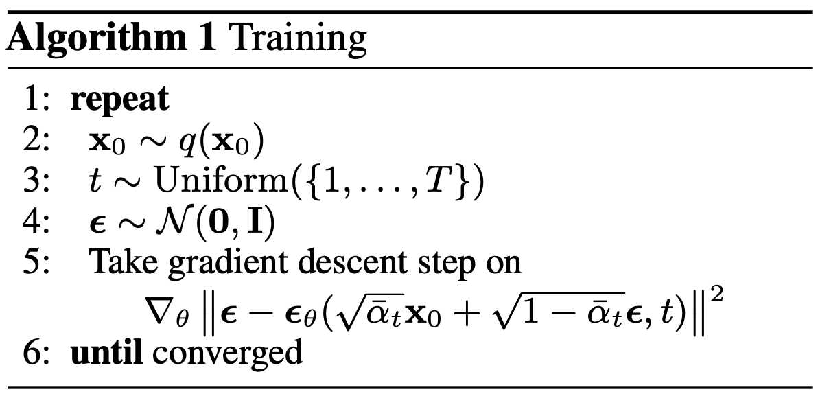
where each training iteration (steps 2 to 5) is implemented by the inner loop below. At the end of every epoch, we use the EMA model to generate and save new images:
    # training loop
    for epoch in range(20):
        sampler.set_epoch(epoch) # shuffle the data differently at every epoch
        for step, x_0 in enumerate(dataloader):
            x_0 = x_0.to(device=device)
            t = torch.randint(0, T, (batch_size,), device=device).long() # Algorithm 1, step 3 (0-indexed)
            noise = torch.randn_like(x_0) # step 4
            x_t = q_sample(x0=x_0, t=t, noise=noise)
            loss = unet_loss(x_t, t, noise) if model_name == 'UNet' else dit_loss(x_0, x_t, t, noise) # step 5
            loss.backward()
            optimizer.step()
            optimizer.zero_grad(set_to_none=True)
            ema.update_parameters(model.module)
            if dist.get_rank() == 0:
                print(f"epoch {epoch}, step {step} loss: {loss.item()}")

        # save images generated with the EMA model
        if dist.get_rank() == 0:
            results_folder = Path("./results")
            results_folder.mkdir(exist_ok = True)
            img = alg2_p_sampling(ema, shape=x_0.shape)
            img = (img + 1) * 0.5 # from [-1,1] to [0,1]
            save_image(img, str(results_folder / f'sample-{epoch}.png'), nrow = batch_size)
Diffusion transformers
With the advancement of Transformers as an important module in sequence-based ML, Scalable Diffusion Models with Transformers introduced diffusion transformers (DiT) as a replacement for U-Net-based diffusion, outperforming it in scaling and sample quality measured by Fréchet inception distance (FID). Because the work presented is based on image diffusion, DiT is based on Vision Transformers (ViTs), that operate on patches of images (Figure 4 in the paper). In practice, DiT operates on patches of the latent representation of the image produced by a pre-trained VAE, as in the latent diffusion models discussed below. ViTs have also been shown to have better scaling properties and accuracy than convolutional neural networks, when trained on large datasets. Moreover, related to DiT scaling, it was shown that (1) DiT Gflops are strongly correlated with FID (more Gflops, lower FID), (2) DiT Gflops are critical to improving performance, and (3) larger DiT models use large compute more efficiently.
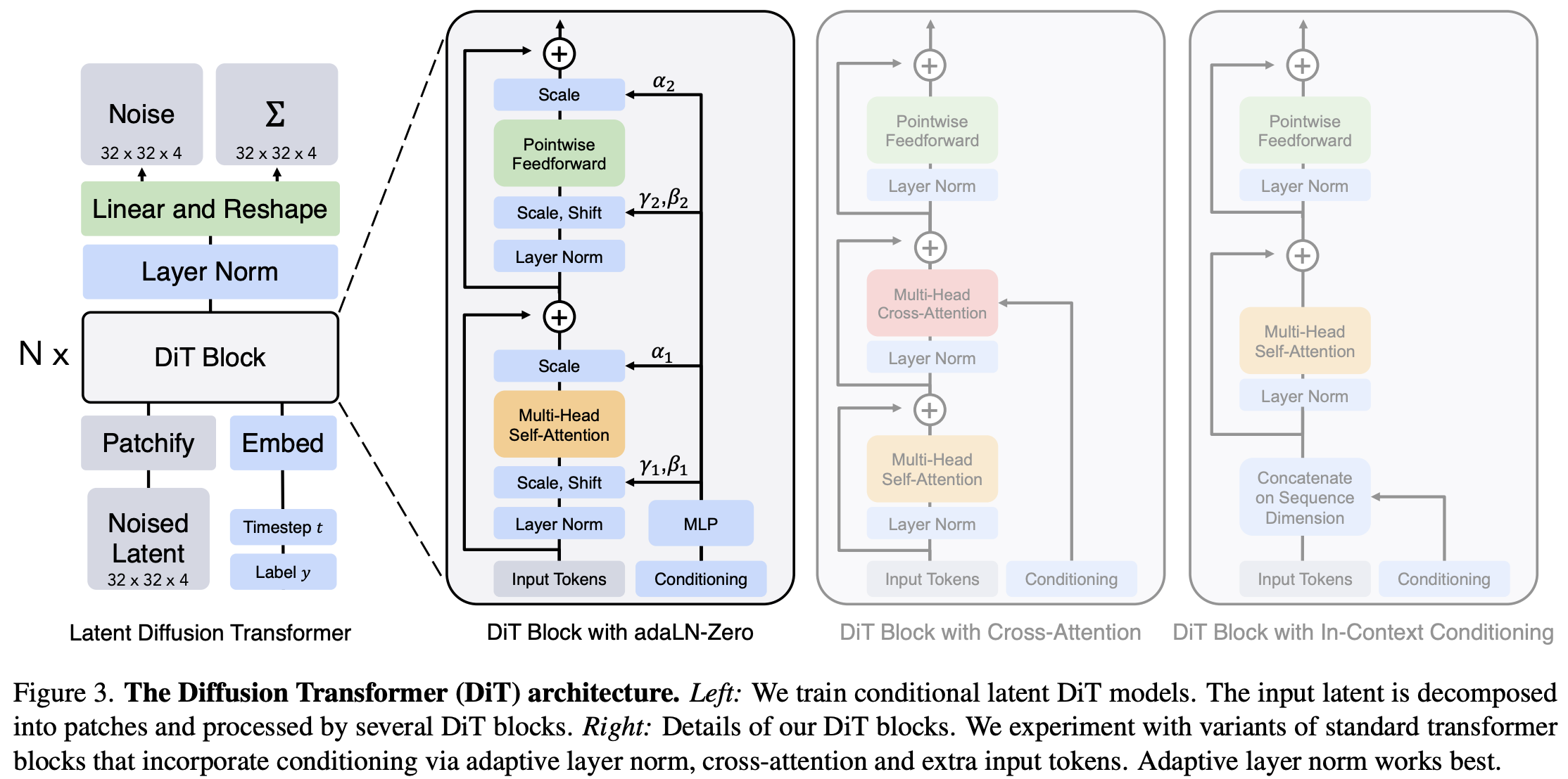
In the adaLN-Zero architecture shown in the diagram, the adaptive layer normalization process applies dynamic conditioning into the model: instead of learning the scale \(\gamma\) and shift \(\beta\) parameters of each layer norm directly, these are regressed by an MLP from the sum of the embeddings of the timestep \(t\) and the class label \(y\) (the conditioning inputs). adaLN-Zero additionally regresses dimension-wise scaling parameters \(\alpha\) that are applied right before each residual connection, and initializes them to zero, so that each DiT block starts as the identity function. Note that these \(\alpha\) and \(\beta\) are unrelated to the \(\alpha_t\) and \(\beta_t\) of the noise schedule.
Here, for the sake of simplicity, we will implement a simple ViT made of a positional embedding layer, a stack of transformer blocks and a decoder. The decoder is a layer-norm and a linear layer that outputs the shape \(p \times p \times 2C\) (ie a predicted noise, and a value that parameterizes the variance, for each channel and pixel of the patch).
To keep our architecture as simple as possible, we will ignore the 4 variants described in DiT block design (in Section 3.2, in-context conditioning, cross-attention block, adaptive layer norm block and adaLN-Zero block): we simply add a timestep embedding to every patch, and use a regular transformer Block (multi-head self-attention followed by a feed-forward network, as in our GPT-lite post). We will also use the regular PyTorch embedding nn.Embedding (a look-up table) instead of the frequency-based positional embeddings (the sine-cosine version). Each token is a flattened image patch, so the embedding size is \(p \times p \times C\).
class DiT(nn.Module):
    """ A Diffusion Transformer (DiT) model """

    def __init__(self, timesteps, num_channels, img_size, patch_size=4, n_blocks=12, num_labels=None):
        super().__init__()
        assert img_size % patch_size == 0, "Image size must be divisible by patch size"
        self.patch_size = patch_size
        n_embd = patch_size*patch_size*num_channels # values per img patch

        # timestep and positional embeddings
        n_pos_emb = (img_size//patch_size)*(img_size//patch_size) # number of patches per image
        self.t_embedding = nn.Embedding(timesteps, n_embd)
        self.pos_embedding = nn.Embedding(n_pos_emb, n_embd)

        # class embeddings, only for a class-conditional model
        self.class_embedding = nn.Embedding(num_labels, n_embd) if num_labels else None

        # DiT blocks
        self.blocks = nn.Sequential(*[Block(n_embd=n_embd) for _ in range(n_blocks)])

        # decoder: "standard linear decoder to do this; we apply the layer norm and linearly decode each token into a p×p×2C tensor"
        self.decoder = nn.Sequential( nn.LayerNorm(nmbd), nn.Linear(n_embd, n_embd*2) )
Then we need to add the boilerplate code that crops the input image into the patches used by the attention module, and that merges the patches back into a single image:
    def patchify(self, x):
        """ break image (B, C, H, W) into patches (B, C, NH, NW, PH, PW) for NH*NW patches of size PHxPW """
        B, C, H, W = x.shape
        x = x.unfold(2, self.patch_size, self.patch_size).unfold(3, self.patch_size, self.patch_size)

        # linearize patches and flatten embeddings: (B, NH*NW, PH*PW*C)
        _, _, NH, NW, PH, PW = x.shape
        x = x.permute(0, 2, 3, 4, 5, 1) # (B, NH, NW, PH, PW, C)
        x = x.reshape(B, NH*NW, PH*PW*C)
        return x, dict(B=B, C=C, H=H, W=W, NH=NH, NW=NW, PH=PH, PW=PW)

    def unpatchify(self, x, shapes):
        """ convert patches (B, NH*NW, PH*PW*C*2) back into the noise ε_θ and the vector v that parameterizes
            the variance Σ_θ, each of shape (B, C, H, W) = (B, C, NH*PH, NW*PW) """
        B, , W, NH, NW, PH, PW, = shapes.values()
        assert x.shape == (B, NH*NW, PH*PW*C*2)
        x = x.reshape(B, NH, NW, PH, PW, C, 2).permute(0, 5, 1, 3, 2, 4, 6) # (B, C, NH, PH, NW, PW, 2)
        x = x.reshape(B, C, NH*PH, NW*PW, 2)
        ε_θ, v = x[...,0], x[...,1]
        assert ε_θ.shape == v.shape == (B, C, H, W) # original shape
        return ε_θ, v
The forward pass then adds the positional and timestep embeddings to the patches (and the class embedding, discussed in the Conditioning s below), and runs the transformer blocks and the decoder:
    def forward(self, x, t, label=None):
        x, shapes = self.patchify(x) # (B, C, H, W) -> (B, N, E), for N patches of E=PH*PW*C values
        B, N, E = x.shape
        x += self.pos_embedding(torch.arange(N, device=x.device)).reshape(1, N, E) # positional embeddings
        x += self.t_embedding(t).reshape(B, 1, E) # timestep embedding, added to all patches of an image
        if label is not None: # class embedding, added to all patches of an image
            x += self.class_embedding(label).reshape(B, 1, E)
        x = self.blocks(x)
        x = self.decoder(x) # (B, N, E) -> (B, N, 2E)
        return self.unpatchify(x, shapes) # ε_θ and v
In this use case, we are also learning the covariance \(\Sigma_\theta\), so we need to optimize the full variational bound \(L\), as \(\mathcal{L}_\text{simple}\) does not depend on \(\Sigma_\theta\). Following Improved DDPM, the model outputs a vector \($ with one value per dimension, that interpolates the variance between its two extreme choices\)\beta_t\(and\)\tilde{\beta}_t$$ (the upper and lower bounds of the reverse process entropy) in the log domain (Eq. 15 in Improved DDPM):
\[\Sigma_\theta(\mathbf{x}_t, t) = \exp \left( v \log \beta_t + (1-v) \log \tilde{\beta}_t \right)\]coded as:
    def learned_Σ_θ(v, t):
        """ Improved DDPM, Equation 15: interpolate log(Σ_θ) between log(β_t) and log(posterior_β_t) """
        fra + 1) / 2 # from the model output in [-1, 1] to [0, 1], as in the official implementation
        log_β_t = torch.log(β)[t][:, None, None, None]
        posterior_log_β_t = posterior_log_β[t][:, None, None, None]
        return torch.exp(frac * log_β_t + (1 - frac) * posterior_log_β_t)
To train it, the authors train \(\epsilon_\theta\) with \(\mathcal{L}_\text{simple}\), as before, and train \(\Sigma_\theta\) with the full bound \(L\), ie they minimize a hybrid loss (Eq. 16 in Improved DDPM):
\[xt{hybrid} = \mathcal{L}_\text{simple} + \lambda L_\text{vlb}\]where \(L_\text{vlb}\) is the variational bound \(L\) of Eq. 5, and \(\lambda = 0.001\) prevents \(L_\text{vlb}\) from overwhelming \(\mathcal{L}_\text{simple}\). A stop-gradient on \(\mu_\theta\) makes \(L_\text{vlb}\) train only \(\Sigma_\theta\). Each term \(L_{t-1}\) of \(L_\text{vlb}\) is a KL divergence between two Gaussians, that has a closed form solution (an alternative implementation can be found in Meta’s DiT implementation), and \(L_0\) is the discretized decoder of Eq. 13. As we sample a single timestep per image, and \(L_\text{vlb}\) sums the terms of \(T\) timesteps, we estimate it as \(T\) times the term of the sampled timestep, measured in bits per dimension as in the paper:
    def dit_loss(x_0, x_t, t, noise):
        """ L_hybrid = L_simple + λ L_vlb, Improved DDPM, Equation 16 """
       ε_θ, v = model(x_t, t)
        Σ_θ = learned_Σ_θ(v, t)
        μ_θ = eq11_μ_θ(x_t, ε_θ.detach(), t) # stop-gradient: L_vlb only trains Σ_θ
        p = torch.distributions.Normal(μ_θ, Σ_θ.sqrt()) # Eq. 1
        q = torch.distributions.Normal(posterior_μ(x_0, x_t, t), torch.exp(0.5 * posterior_log_β[t][:, None, None, None])) # Eq. 6
        kl = torch.distributions.kl_divergence(q, p).mean(dim=(1, 2, 3)) # L_{t-1}
        nll = eq13_decoder_nll(x_0, p).mean(dim=(1, 2, 3)) # L_0
        L_= torch.where(t == 0, nll, kl) / math.log(2) # per sample, in bits per dimension (t=0 is the paper's t=1)
        L_simple = F.mse_loss(ε_θ, noise)
        return L_simple + T / 1000 * L_vlb.mean() # λ = 1/1000, times T as L_vlb sums the losses of T timesteps
In fact, the paper implements a conditional diffusion model that takes as input extra information such as class \(c\), and the reverse process becomes \(p_\theta(\mathbf{x}_{t-1} \mid \mathbf{x}_t, c)\), where \(\epsilon_\theta\) and \(\Si_\theta\) are conditioned on \(c\). We’ll look at that next.
Conditioning
The previous model learns to generate samples from the data distribution. On a dataset like CIFAR-10 that has 10 classes of objects, it would generate an image from a random class, with no way for us to pick which one. So it would be helpful to add some guidance that tells the model which class we want to generate. We can do this by adding conditional information.
The previous implementation was generating/sampling new images from a diffusion process. One can add conditioning for the class id, input text, guiding image, or other information we want to train on.
Our DiT takes the class label as optional additional information: when created with a number of labels num_labels, it learns a class embedding that is added to all patches of an image, just like the timestep embedding:
    def __init__(self, timesteps, num_channels, img_size, patch_size=4, n_blocks=12, num_labels=None):
        # [...]
        # class embeddings, only for a class-conditional model
        self.class_embedding = nn.Embedding(num_labels, n_embd) if num_labels else None
        # [...]

    def forward(self, x, t, label=None):
        # [...]
        if label is not None: # class embedding, added to all patches of an image
            x += self.class_embedding(label).reshape(B, 1, E)
        # [...]
Our training script trains an unconditional model, but a class-conditional one can be trained by also passing the CIFAR10 label of each image to the model.
Another interesting feature that improves quality is classifier-free guidance, that for brevity will be omitted. Finally, conditioning allows us to train diffusion models with text, image or audio as the input signal.
Video diffusion and 3D attention
Running diffusion directly on pixels is already expensive for high-resolution images. This led to the creation of the latent diffusion model, where diffusion is applied on the latent space of pretrained autoencoders (e.g. a VAE) instead of on the image directly. This reduces the cost of training on high-resolution images by working on their compressed representation instead. As diffusion moved towards the domain of video, the large amount of data per sample made this compression even more important, and video models now compress their input in both the spatial and temporal dimensions:

An overview of the latent space compression in SORA. The pre-processing step “turns videos into [visual] patches by first compressing videos into a lower-dimensional latent space and subsequently decomposing the representation into spacetime patches”. Source: Video generation models as world simulators, OpenAI
The other challenge in video datasets is the attention: how do we correlate image patches across the spatial domain in a picture, and across the time domain? Given an input of shape \(B \times T \times H \times W \times C\) (batch, number of frames, height, width and channels; here \(T\) is the number of frames, not of diffusion steps), there are two main approaches:
- a spatial attention that converts an input \(B \times T \times H \times W \times C\) into \((B * T ) \times (H * W) \times C\) to perform attention of patches within the same frame, and then follow it by a temporal attention that converts it into \((B * H * W) \times T \times C\) that performs attention of the same patch across time. Doing this across several U-Net or DiT blocks correlates patches across both space and time.
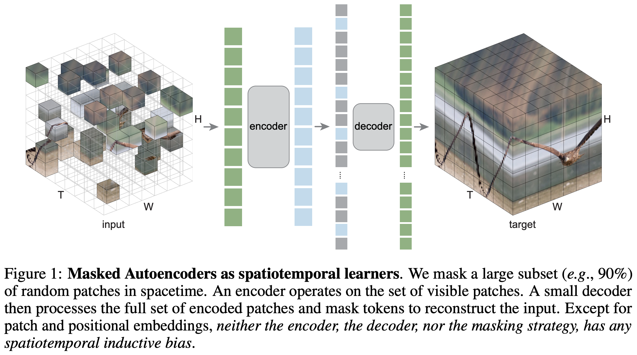
- a full 3D attention, where we collect all patches of all frames and use them as the sequence dimension in the attention ie converting an input of shape \(B \times T \times H \times W \times C\) into \(B \times (T * H * W) \times C\). This leads to a very large sequence dimension, which is an issue because computation in the attention mechanism grows quadratically with the sequence length. However, Masked Autoencoders Are Scalable Vision Learners showed that masked autoencoders (MAE) are scalable self-supervised learners for computer vision that only need to encode a random subset of the patches (25% on images), and Masked Autoencoders As Spatiotemporal Learners extended it to videos, where only 10% of the \(T * H * W\) spacetime patches are needed. Patch n’ Pack: NaViT, a Vision Transformer for any Aspect Ratio and Resolution also uses random token dropping, together with sequence packing, to speed up training.
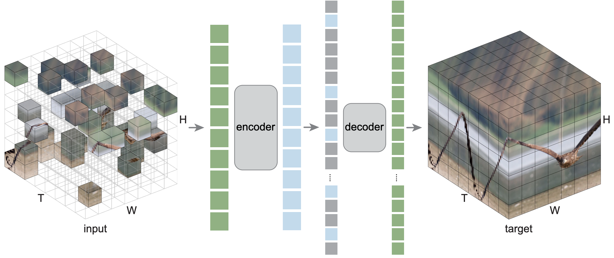
An illustration of a masked autoencoder randomly picking 10% of the spacetime patches of a video, retaining enough representative power to reconstruct the original video. Source: Masked Autoencoders As Spatiotemporal Learners
Further Reading
Here are some examples of U-Net based diffusion models for text-to-image and text-to-video tasks:
Imagen: Photorealistic Text-to-Image Diffusion Models with Deep Language Understanding
A U-Net based text-to-image diffusion model, where “key discovery is that generic large language models (e.g. T5), pretrained on text-only corpora, are surprisingly effective at encoding text for image synthesis: increasing the size of the language model in Imagen boosts both sample fidelity and image-text alignment much more than increasing the size of the image diffusion model”.
Stable Video Diffusion: Scaling Latent Video Diffusion Models to Large Datasets
Presents a U-Net based diffusion model for text-to-video and (text-to-)image-to-video generation. It is trained in 3 stages: (1) text-to-image pretraining of a diffusion model, (2) video pretraining on a large dataset at low resolution, and (3) high-resolution video finetuning on a much smaller dataset with higher-quality videos. It also emphasizes the importance and methods for data curation: e.g. avoiding cutscenes or static scenes, removing videos with a large amount of written text. To train on videos, they use the method presented in Align your Latents: High-Resolution Video Synthesis with Latent Diffusion Models, that adds temporal layers to a pre-trained image model:
first pre-train the diffusion model on images only; then, turn the image generator into a video generator by introducing a temporal dimension to the latent space diffusion model and fine-tuning on encoded image sequences, i.e., videos.
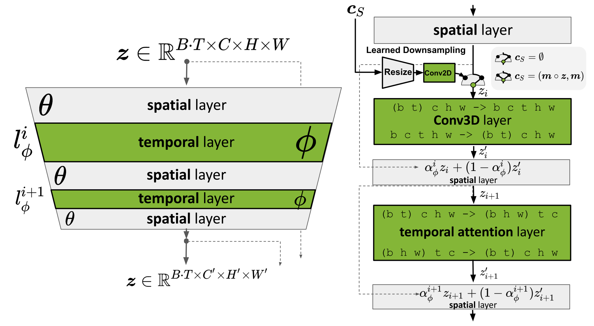
Left: We turn a pre-trained LDM into a video generator by inserting temporal layers that learn to align frames into temporally consistent sequences. During optimization, the image backbone \(\theta\) remains fixed and only the parameters \(\phi\) of the temporal layers \(l^i_\phi\) are trained, cf. Eq. (2). Right: During training, the base model \(\theta\) interprets the input sequence of length \(T\) as a batch of images. For the temporal layers \(l^i_\phi\), these batches are reshaped into video format. Their output \(z'\) is combined with the spatial output \(z\), using a learned merge parameter \(\alpha\). During inference, skipping the temporal layers (\(\alpha^i_\phi=1\)) yields the original image model. For illustration purposes, only a single U-Net Block is shown. \(c_S\) is optional context frame conditioning, when training prediction models (Sec. 3.2). Source and caption: Align your Latents: High-Resolution Video Synthesis with Latent Diffusion Models.
Animate Anyone: Consistent and Controllable Image-to-Video Synthesis for Character Animation
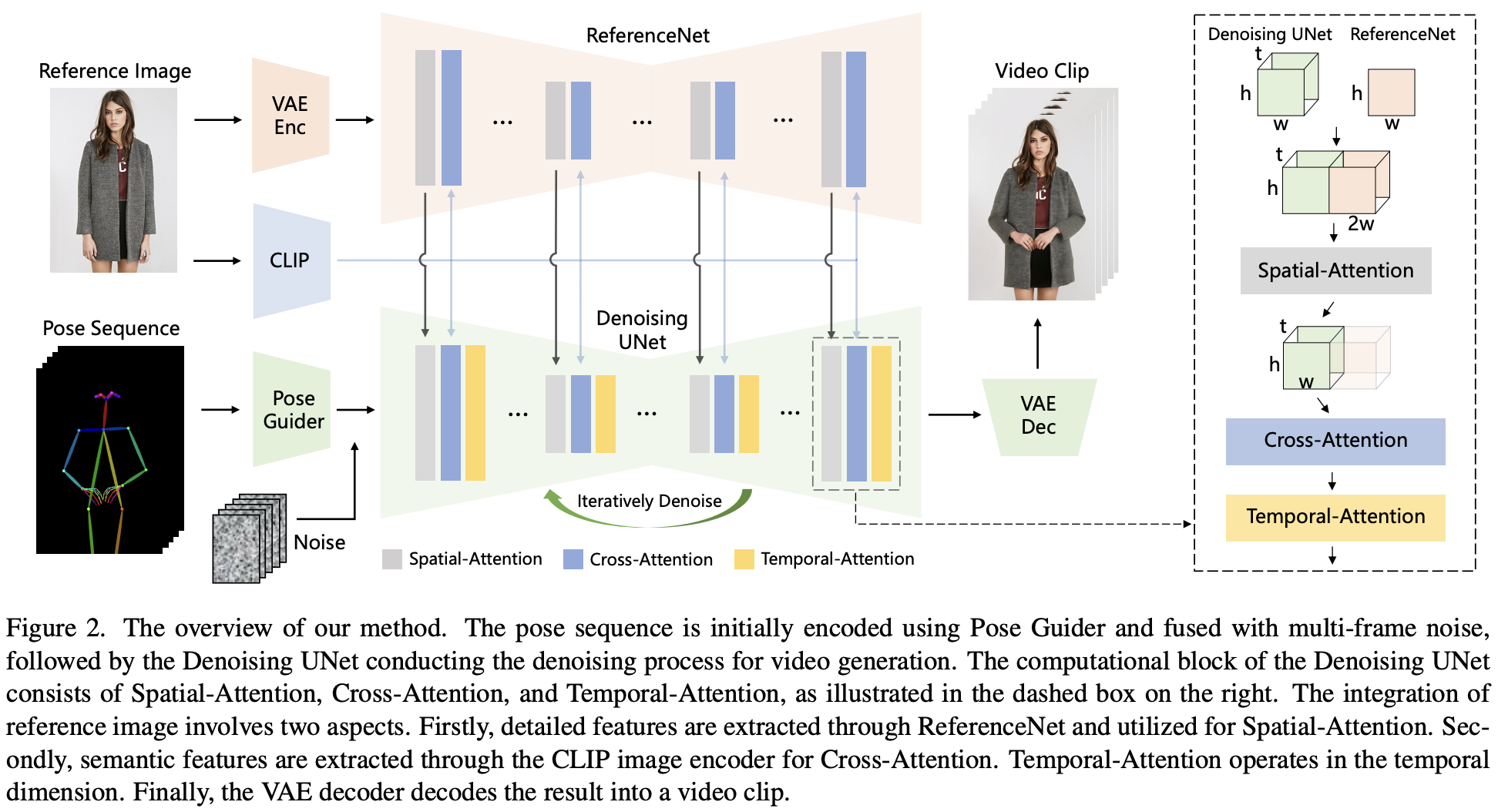
A U-Net based diffusion model that takes as input a reference image (photo of a human) and a video of a moving human annotation (stick man, the pose sequence) and outputs the video that animates the human with the movements of the stick man. The reference image is encoded with VAE and CLIP embeddings. The model structure includes 2 U-Nets: the reference U-Net that merges detail features via spatial attention and a denoising U-Net that generates the video, conditioned on the pose sequence (encoded by a lightweight pose guider).
Spatio-temporal attention is achieved by a spatial attention that converts an input \(B \times T \times H \times W \times C\) into \((B * T ) \times (H * W) \times C\) to perform attention of patches within the same frame, followed by a temporal attention that converts it into \((B * H * W) \times T \times C\) and performs attention of the same patch across time.
CyberHost: Taming Audio-driven Avatar Diffusion Model with Region Codebook Attention
CyberHost is a U-Net based diffusion model that takes audio as input and generates valid human movements. The novelty, compared to Animate Anyone, is the Region Codebook Attention which improves the generation quality of facial and hand animations by integrating fine-grained local features with learned motion pattern priors.
Emu: Enhancing Image Generation Models Using Photogenic Needles in a Haystack
Demonstrates the importance of fine-tuning text-to-image models on a small dataset of very high quality images in order to achieve superior model quality: “in order to align the model towards highly aesthetic generations, quality matters significantly more than quantity in the fine-tuning dataset”.
And here are some examples of DiT inspired conditional diffusion models:
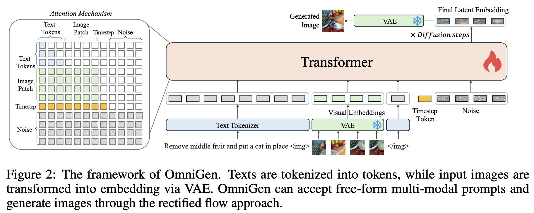
OmniGen: Unified Image Generation
OmniGen is a diffusion model made only of a VAE and a transformer (initialized from the Phi-3 LLM), able to perform several image generation tasks: text-to-image, image editing, subject-driven generation and visual-conditional generation. Text input is tokenized, and image inputs are transformed into embeddings via a VAE.
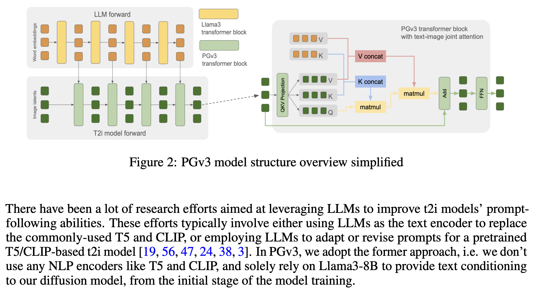
Playground v3: Improving Text-to-Image Alignment with Deep-Fusion Large Language Models
A text-to-image diffusion model, that replaces the commonly used T5 and CLIP for input text encoding with the latents of a decoder-only LLM (Llama3-8B).
Here is some work on video diffusion and 3D attention:
Patch n’ Pack: NaViT, a Vision Transformer for any Aspect Ratio and Resolution
NaViT (Native Resolution ViT) uses sequence packing during training to process inputs of arbitrary resolutions and aspect ratios. This is done by packing multiple patches from different images into a single sequence (the “Patch n’ Pack” method) which enables variable resolution while preserving the aspect ratio.
CogVideoX: Text-to-Video Diffusion Models with An Expert Transformer
CogVideoX is a large-scale DiT model for text-to-video generation. Model input is a pair of video and text. Text input is encoded with5. Video input is passed through a 3D causal VAE that compresses the video into the latent space, and then all video patches are unfolded into a long sequence. Text and video embeddings are then concatenated as input, and passed to a stack of expert transformer blocks. The model output is then unpatchified to restore the original latent shape, and decoded using a 3D causal VAE to reconstruct the video. The attention is provided by a 3D attention model (that unfolds all patches of all frames) instead of a separate spatial and temporal attention.
Latte: Latent Diffusion Transformer for Video Generation
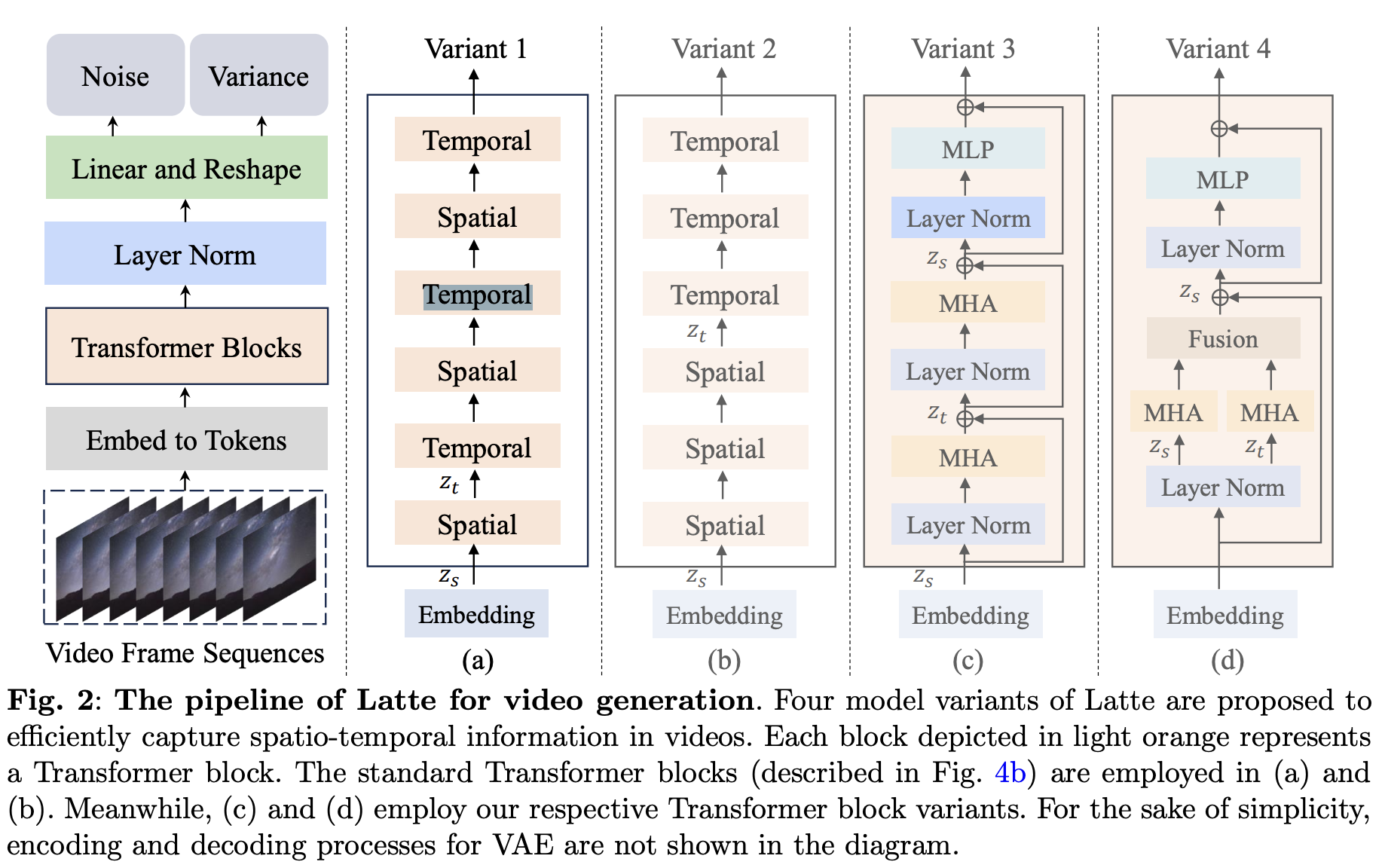
Latte is a DiT-based text-to-image and text-to-video diffusion model. Latte first extracts spatio-temporal tokens from input videos and then adopts a series of Transformer blocks to model video distribution in the latent space. The paper experiments with several methods for embedding, clip patch embedding, model variants, timestep-class information injection, temporal positional embedding, and learning strategies, and provides a report. As an example, it tests four variants of 3D transformer block: (1) with spatial Transformer blocks and temporal Transformer blocks, (2) a “late fusion” approach to combine spatial-temporal information, that consists of an equal number of Transformer blocks as in Variant 1, (3) that “initially computes self-attention only on the spatial dimension, followed by the temporal dimension, and as a result, each Transformer block captures both spatial and temporal information”, and (4) one that uses different attention heads to handle tokens separately in spatial and temporal dimensions.
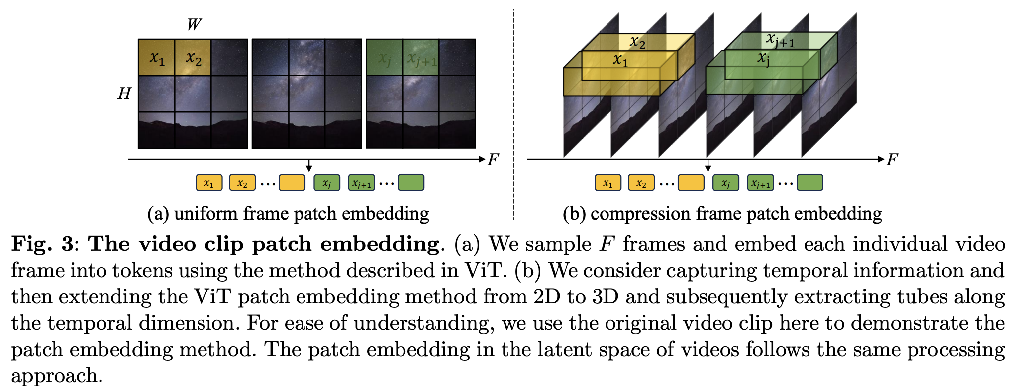
The paper also analyses 2 distinct methods for video patch embedding: (1) collect all patches of a frame, and then collect the patches for the following frame etc, as in ViT, (2) extracting patches in the temporal dimension as well (in a “tube”) and move that tube in the spatial dimension:
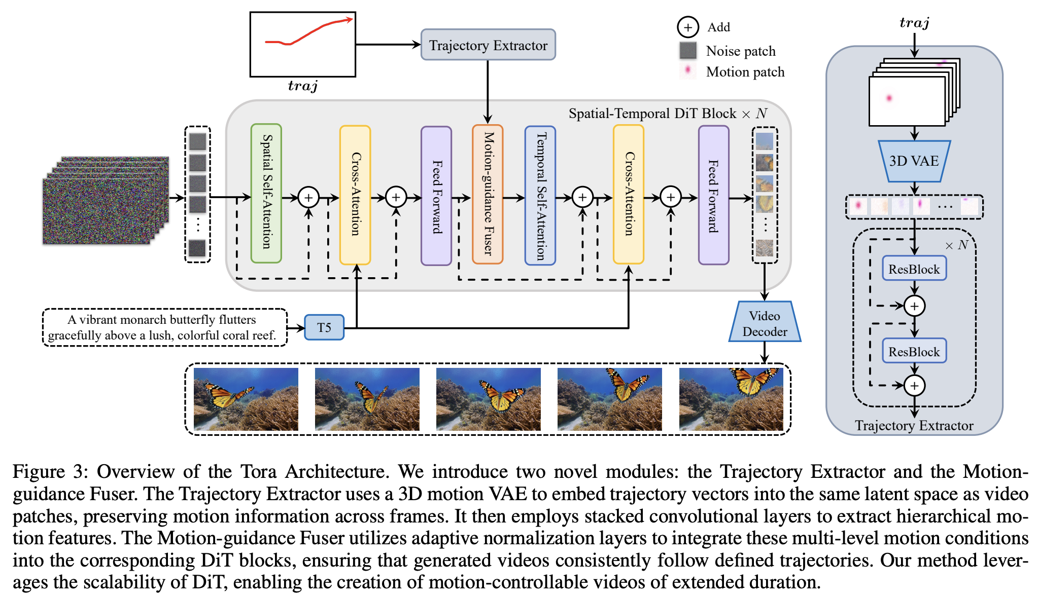
Tora: Trajectory-oriented Diffusion Transformer for Video Generation (webpage)
Tora is capable of generating videos guided by trajectories, images, texts, or combinations thereof. “Spatial-Temporal Diffusion Transformer (ST-DiT) from OpenSora as its foundational model”, ie a spatial attention followed by a temporal attention, similar to variant 3 in Latte (above). The big advantage of using ST-DiT compared to 3D attention is that it saves on computation and it can use pre-trained text-to-image models. “The trajectory encoder converts the trajectory into motion patches, which inhabit the same latent space as the video patches”. Text encoding is provided by T5.
Masked Autoencoders As Spatiotemporal Learners (github)
It applies Masked AutoEncoders (MAE) to the video domain, demonstrating high compute efficiency:
We randomly mask out spacetime patches in videos and learn an autoencoder to reconstruct them in pixels. Interestingly, we show that our MAE method can learn strong representations with almost no inductive bias on spacetime (only except for patch and positional embeddings), and spacetime-agnostic random masking performs the best. We observe that the optimal masking ratio is as high as 90% (vs. 75% on images [31]), supporting the hypothesis that this ratio is related to information redundancy of the data. A high masking ratio leads to a large speedup, e.g., > 4× in wall-clock time or even more.
And here is some work on multi-dimensional parallelism for arge-scale models such as SORA:
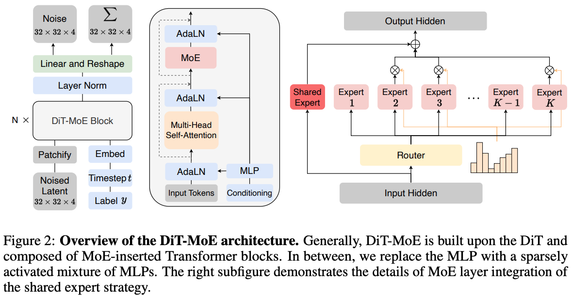
Scaling Diffusion Transformers to 16 Billion Parameters
Presents DiT-MoE, a sparse Mixture of Experts (MoE) version of DiT, delivering good scaling properties, a performance comparable to dense DiTs, and highly optimized inference.
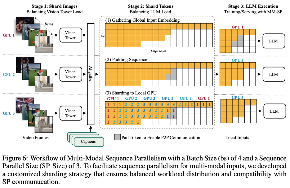
LongVILA: Scaling Long-Context Visual Language Models for Long Videos
LongVILA details a pipeline of 5 steps for training long-context visual-language models. The first 3 stages are multi-modal alignment, large-scale pre-training and short supervised fine-tuning from VILA: On Pre-training for Visual Language Models. Stage 4 is context extension for LLMs, by increasing the sequence length of input samples (ie curriculum learning) up to 262K tokens. In Stage 5, the model is fine-tuned for long video understanding with Multi-Modal Sequence Parallelism (MM-SP) based on LoongTrain: Efficient Training of Long-Sequence LLMs with Head-Context Parallelism.
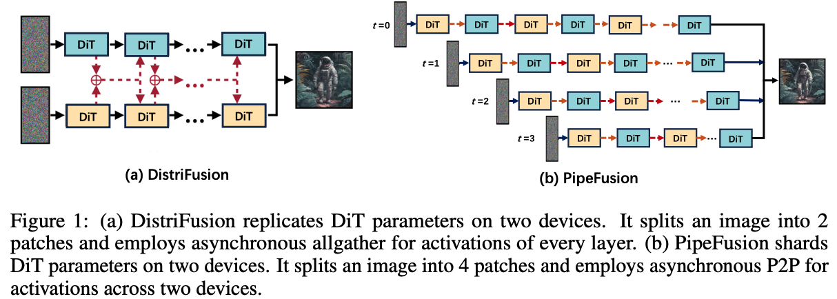
PipeFusion: Displaced Patch Pipeline Parallelism for Inference of Diffusion Transformer Models and xDiT github.
PipeFusion splits images into patches and distributes the network layers across multiple devices. It employs a pipeline parallel manner to orchestrate communication and computations. xDiT is a parallel inference engine of DiTs using Universal Sequence Parallelism (including Ulysses attention and Ring attention), PipeFusion, and hybrid parallelism. It applies and benchmarks xDiT on the following DiT implementations: CogVideo, Flux, Latte, HunyuanDiT, Stable Diffusion 3, PixArt-Sigma, PixArt-alpha.
OpenSORA implementation from HPC AI Tech
An attempt to create an open-source implementation of SORA. The details below refer to version 1.2, and were collected from the docs section, particularly the technical reports:
- acceleration provided by kernel optimization (flash attention), fused layernorm kernel, and ones compiled by colossalAI. Sequence parallelism is based on Ulysses, and used only for inference;
- Spatio-temporal attention is provided by ST-DiT instead of full 3D attention, as ST-DiT is more (compute) efficient as the number of frames increases.
- Data processing is explained in the Data Processing and Datasets pages;
- Texts are encoded by T5 and videos by VAE: the 2D VAE is initialized with SDXL’s VAE, and the 3D VAE follows the architecture of Magvit-v2. See the VAE Report for additional info. The video compression network used was an 83M 2D VAE in the previous version, compressing only the spatial dimension by 8x8, with 1 frame picked in every 3 (to reduce the temporal dimension). To improve quality, in version 1.2 the authors first compress the video in the spatial dimension by 8x8 times, then compress the video in the temporal dimension by 4x times.
- The VAE training includes 3 stages: (1) freeze the 2D VAE in order to train features from the 3D VAE similar to the features from the 2D VAE; (2) remove the identity loss and just learn the 3D VAE; and (3) train the whole VAE to reconstruct the original videos. The diffusion model is then trained with a curriculum of increasing data quality, in three stages, to better utilize compute (source);
- It used rectified flow instead of DDPM for diffusion (source).
Movie Gen: A Cast of Media Foundation Models research paper
One of the most detailed technical reports of a very large transformer-based video generation model (a LLaMa3-like transformer trained with flow matching, instead of a DiT trained with diffusion), trained on up to 6,144 H100 GPUs, able to solve multiple tasks: text-to-video synthesis, video personalization, video editing, video-to-audio generation, and text-to-audio generation. “The largest video generation model is a 30B parameter transformer trained with a maximum context length of 73K video tokens, corresponding to a generated video of 16 seconds at 16 frames-per-second”. Section 3.1.6 “Model scaling and training efficiency” (with more details in Appendix A.2) details the combination of 4 parallelism methods: Fully Sharded Data Parallelism, Tensor parallelism, Sequence parallelism and Context Parallelism. Also includes details on the overlapping of communication and computation, and the usage of activation checkpointing for improved memory efficiency.