Inference optimization (1): caching, continuous batching, attention, and distillation
Previously, in Distributed training of a large GPT model with DeepSpeed, we focused on training a very large model on a distributed network of GPUs. The aim was to reduce training runtime via increased parallelism, and to increase model accuracy by increasing model size. In this post, we look at the other end of the model lifecycle: inference. The goal is to generate text as fast and as cheaply as possible, with a small memory footprint, and with little or no loss of quality. This matters for real-time and embedded systems, and for any service where the cost per generated token adds up.
This is the first of two posts on inference optimization. Just like in the previous posts, we use the GPTlite model, a small variant of the GPT-2 model that generates text by predicting the next character in a sequence. The code of each technique is in its own file, which imports GPTlite, and the post shows only the parts that matter, in collapsible sections. All the code is in the repository of this post, together with inference_utils.py, a few helpers shared by all files (model loading, timing and evaluation). GPTlite is tiny, so some techniques designed for billion-parameter models give small or no speedups at our scale; when that happens, we explain why.
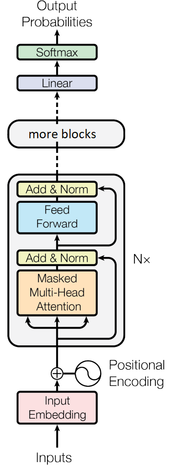
This post covers:
- Background: how a GPT generates text, and where the time goes.
- Caching: the KV cache, prefix caching and semantic caching.
- Batching and scheduling: continuous batching, PagedAttention, chunked prefill, disaggregation and parallelism.
- Faster attention: FlashAttention, smaller KV caches, and quantized, sparse and linear attention.
- Distillation and pruning: smaller models that behave like larger ones.
The second part covers speculative decoding and multi-token prediction, quantization, kernel fusion and compilers, and architectures built for fast inference.
Background: how a GPT generates text, and where the time goes
Prefill and decode
A GPT model generates text autoregressively: it reads the prompt, predicts the next token, appends it to the input, and repeats. Inference therefore has two phases that behave very differently:
- Prefill processes all the prompt tokens in a single forward pass. The tokens are processed in parallel, so the GPU performs large matrix-matrix multiplications and is compute-bound. Prefill ends with the first generated token, so its duration is the time to first token (TTFT).
- Decode generates the remaining tokens, one forward pass per token. Each pass processes a single new token per sequence, so the GPU performs matrix-vector multiplications: it reads every weight of the model from memory to do very little arithmetic with it. Decode is memory-bandwidth-bound, and the duration of each step is the time per output token (TPOT), also called inter-token latency.
A quick calculation shows why decode is memory-bound. In a matrix-vector product, each weight (2 bytes in a 16-bit format) is used for one multiplication and one addition per sequence in the batch. With a batch of \(B\) sequences, the GPU performs about \(B\) floating point operations (FLOPs) per byte read from memory. An NVIDIA H100 delivers about 1,000 TFLOP/s of 16-bit compute and 3.35 TB/s of memory bandwidth, so it needs about 300 FLOPs per byte read to keep its compute units busy. With any batch smaller than a few hundred sequences, the GPU spends most of the decode time waiting for memory.
This observation explains most of this post. Almost every decode optimization does one of three things: it reads fewer bytes per token (quantization, smaller KV caches, smaller models), it does more useful work per byte read (batching, speculative decoding), or it removes overheads around the math (kernel fusion, CUDA graphs, better scheduling).
Throughout the post, we look at:
- TTFT and TPOT, the latencies a user perceives;
- throughput, the total number of tokens generated per second across all requests;
- peak memory;
- quality, measured as the validation loss (or perplexity) of the model.
Latency and throughput pull in opposite directions: larger batches increase throughput, but make each step slower, so every user waits a little longer for each token.
Where the compute goes: MLP versus attention
For a model of width \(d\) (the embedding size) and a context of \(n\) tokens, each layer spends, for every token:
- about \(8d^2\) FLOPs in the query, key, value and output projections of the attention block;
- about \(16d^2\) FLOPs in the MLP (the feed-forward network), whose hidden layer has size \(4d\);
- about \(4nd\) FLOPs computing the attention scores \(QK^T\) and the weighted sum of the values.
The first two terms do not depend on the context length; the third grows with every token in the context. Attention becomes the dominant cost when \(4nd > 24d^2\), i.e., when the context is longer than about \(6d\) tokens. For a typical 8B-parameter model (\(d = 4096\)), that is around 25,000 tokens; smaller models reach this point sooner. For short prompts the MLP dominates; for long documents, long conversations and long reasoning traces, attention does.
Memory follows the same pattern. The model weights are read once per decode step and shared by all the sequences of the batch, while each sequence keeps its own cache of attention keys and values (next section) that grows with every token. For long contexts and large batches, reading these caches dominates the memory traffic of each decode step.
Caching
There are three kinds of inference caching, each operating at a different layer of the stack (this three-layer view is adapted from this guide):
- KV caching stores the attention keys and values computed during a single request, so that the model does not recompute them at every decode step. Every serving engine uses it.
- Prefix caching extends KV caching across requests. When different requests share the same leading tokens, such as a system prompt, a reference document, few-shot examples or the previous turns of a conversation, the keys and values of that shared prefix are computed once and reused. It is also called prompt caching or context caching.
- Semantic caching is an application-level cache that stores complete input/output pairs and retrieves them by meaning. Unlike prefix caching, which reuses internal attention states, semantic caching skips the model call entirely when a sufficiently similar query was answered before.
These are complementary layers, not alternatives. KV caching is always on, prefix caching is the highest-leverage optimization for most production applications, and semantic caching pays off when many queries are similar. In short: the KV cache reuses work within one generation, prefix caching reuses work across requests, and semantic caching reuses whole answers.
KV cache
In the attention layer, the query of the new token attends to the keys and values of all previous tokens. In a causal model, the keys and values of past tokens never change, since token \(i\) only depends on the tokens before it. Without a cache, each decode step recomputes the keys and values of the whole sequence, so generating \(n\) tokens costs \(O(n^2)\) work in the projections and MLPs and \(O(n^3)\) in attention. With a cache, each step only computes the query, key and value of the new token, appends the new key and value to the cache, and attends over all cached ones: \(O(n)\) and \(O(n^2)\) in total. Queries do not need to be cached, because the query of a past token was only needed to compute the output at that past position.
The price is memory. For every token, every layer stores a key and a value vector per key-value head:
\[\text{KV cache size} = 2 \times n_\text{layers} \times n_\text{kv heads} \times d_\text{head} \times \text{bytes per value} \times \text{sequence length} \times \text{batch size}\]For example, Llama-3-8B (32 layers, 8 key-value heads of size 128, 16-bit values) needs 128 KB per token, or 1 GB for a single sequence of 8K tokens. This memory, not compute, often limits how many sequences can be batched together, which is why many techniques in this post shrink the KV cache.
Two implementation details matter in practice:
- A dynamic cache grows by concatenating the new keys and values to the cache at every step. This is simple, but every concatenation allocates a new tensor and copies the whole cache. A static cache preallocates a buffer for the maximum sequence length and writes each new entry in place. Static shapes also allow CUDA graphs to remove launch overheads (see part 2).
- GPTlite uses learned absolute positional embeddings and a context window of
seqlentokens. When a sequence grows longer thanseqlen, the model without a cache slides its window and re-encodes the lastseqlentokens at positions 0 toseqlen-1, at every step. A KV cache cannot reproduce this, because the cached keys and values were computed at their original positions and with the context available back then. The model with a cache therefore matches the original model exactly for the firstseqlentokens only. Our implementation keeps the lastseqlenkeys and values, and gives every new token the last position,seqlen-1: generation can continue past the context window, but its output no longer matches the original model. Models with relative positional encodings, such as RoPE, handle a sliding window more gracefully, but keeping only the most recent tokens still changes the output (see sparse attention below).
Our implementation also accepts several new tokens on top of a cache, which prefix caching and speculative decoding need: the causal mask is shifted, so that each new token attends to all the cached tokens and to the new ones up to itself.
The following code implements a KV cache in GPTlite. The full code is in gptlite_kvcache.py (the model) and main_kvcache.py (text generation with and without the cache):
Show code
# gptlite_kvcache.py: Sq new tokens attend to the cached keys and values, and to the new ones up to themselves
def scaled_dot_product_attention_kv_cache(Q, K, V, causal_mask=True, dropout=None):
    scores = torch.matmul(Q, K.transpose(-2, -1)) / (K.size(-1) ** 0.5)  # [B, H, Sq, Sk]
    Sq, Sk = Q.size(2), K.size(2)
    if causal_mask and Sq > 1:
        mask = torch.ones(Sq, Sk, device=Q.device).tril(diagonal=Sk - Sq)
        scores = scores.masked_fill(mask == 0, float('-inf'))
    # ...

class MultiHeadAttention_KVCache(nn.Module):

    def forward(self, x, kv_cache=None, causal_mask=True, max_seqlen=None):
        B, S, _ = x.shape
        H, D = self.n_heads, self.d_head

        # Compute Q, K, V of the new tokens
        q = self.query_proj(x).view(B, S, H, D).transpose(1, 2)  # [B, H, S, D]
        k = self.key_proj(x).view(B, S, H, D).transpose(1, 2)
        v = self.value_proj(x).view(B, S, H, D).transpose(1, 2)

        # If a cache is provided, prepend the past keys and values
        if kv_cache is not None:
            past_keys, past_values = kv_cache
            k = torch.cat([past_keys, k], dim=2)  # [B, H, S_past + S, D]
            v = torch.cat([past_values, v], dim=2)
            # Keep at most the last max_seqlen keys and values
            if max_seqlen is not None and k.size(2) > max_seqlen:
                k = k[:, :, -max_seqlen:, :]
                v = v[:, :, -max_seqlen:, :]

        out = scaled_dot_product_attention_kv_cache(q, k, v, causal_mask=causal_mask,
                                          dropout=self.dropout if self.training else None)
        # ...
        new_cache = (k, v)
        return out, new_cache

# gptlite_kvcache.py: the new tokens follow the cached ones
class GPTlite_KVCache(nn.Module):

    def forward(self, x, kv_cache=None, max_seqlen=None):
        B, T = x.shape
        if kv_cache is not None and kv_cache[0] is not None:
            S_past = kv_cache[0][0].size(2)  # S_past from first layer's past_keys
            positions = torch.arange(S_past, S_past + T, device=x.device).clamp(max=self.seqlen - 1)
            positions = positions.unsqueeze(0).expand(B, T)
        else:
            positions = torch.arange(T, device=x.device).unsqueeze(0).expand(B, T)
        # ...
        # Process through blocks: one cache per layer
        new_caches = []
        for block, layer_cache in zip(self.blocks, kv_cache):
            x, new_cache = block(x, kv_cache=layer_cache, max_seqlen=max_seqlen)
            new_caches.append(new_cache)
        # ...
        return x, new_caches

# main_kvcache.py: process the prompt once (prefill), then one new token per step (decode)
def generate_kvcache(model, prompt, n_tokens, seqlen, kv_cache=None):
  logits, kv_cache = model(prompt, kv_cache=kv_cache, max_seqlen=seqlen)
  tokens = prompt
  for i in range(n_tokens):
    next_token = torch.argmax(logits[:, -1], dim=-1, keepdim=True)
    tokens = torch.cat([tokens, next_token], dim=-1)
    if i < n_tokens - 1:
      logits, kv_cache = model(next_token, kv_cache=kv_cache, max_seqlen=seqlen)
  return tokens
Prefix caching
Many requests start with the same tokens: a system prompt, tool definitions, a long document that users ask several questions about, or the history of a conversation. Prefix caching keeps the keys and values of these tokens after a request finishes, so that the next request starting with the same tokens skips their prefill and only processes its new part. The first token arrives much sooner, and the GPU is free for other work. Hosted LLM APIs offer this as prompt caching or context caching, and bill cached input tokens at a discount.
Why the prefix must match exactly. It is tempting to look for similar prompts, e.g., with a vector database, instead of identical ones. This does not work for attention states. The key and value of token \(i\) depend on all the tokens before it, through every layer of the model. Two prompts that differ in a single early token, even if they mean the same, have different keys and values for every token after that difference. Reusing the cache of a similar prompt would silently feed the model a different context than the one the user sent. Exact matching makes prefix caching lossless: the output is identical to running the model without the cache. It is also cheap: a hash or tree lookup, instead of computing an embedding and searching a vector index. Similarity search does make sense one level up, where whole answers are reused: that is semantic caching, below.
Prefixes, not substrings. For the same reason, only a prefix can be reused, i.e., the first \(N\) tokens of the prompt. A paragraph in the middle of a prompt has different keys and values depending on what comes before it. Matching is done on token IDs, not on raw text, so the same text tokenized differently (e.g., with an extra space) is a miss. Research systems reuse non-prefix chunks approximately: CacheBlend precomputes the cache of each retrieved document independently and recomputes a small fraction of tokens to restore the attention between documents, and Prompt Cache reuses precomputed modules of prompts written in a structured template.
How the lookup works. vLLM splits the cache into fixed-size blocks (e.g., 16 tokens) and identifies each full block by a hash of its tokens combined with the hash of the previous block. The chain of hashes identifies the whole prefix, so a lookup walks the blocks from the start of the prompt and stops at the first miss. SGLang’s RadixAttention stores all cached sequences in a radix tree (a compressed prefix tree), finds the longest prefix shared with each new request, and evicts the least recently used leaves when memory runs out.
What is kept. The KV cache holds the keys and values of every token processed so far, in every layer: the prompt and all the generated tokens, not only the last decode step, since every new token attends to all of them. When a request finishes, its blocks are not freed right away: they stay in memory, marked as reusable, until the memory is needed for something else. Generated tokens are cached too, which is what makes multi-turn chat fast: the prompt of the next turn is the previous prompt, plus the previous answer, plus the new message.
Practical consequences. Put the static content first (system prompt, tools, documents) and the variable content last (the user’s question, timestamps): anything that changes early in the prompt invalidates the cache for everything after it. At scale, engines offload cached blocks to CPU memory, SSDs or a shared store to keep more prefixes available (e.g., LMCache and Mooncake), and cache-aware routers send each request to the replica that already holds its prefix.
The following code implements prefix caching on top of the KV cache: the keys and values of a shared prefix are computed once, and reused by every request. The full code is in main_prefix_cache.py, which also checks that the outputs are the same as without prefix caching:
Show code
# without prefix caching: every request processes the shared prefix again
for request in requests:
  generate_kvcache(model, torch.cat([prefix, request[None]], dim=1), n_tokens, seqlen)

# with prefix caching: the keys and values of the prefix are computed once and reused by every
# request. Attention creates new tensors when it appends to the cache (torch.cat), so the prefix
# cache is never modified and can be shared by all requests
_, prefix_cache = model(prefix)
for request in requests:
  generate_kvcache(model, request[None], n_tokens, seqlen, kv_cache=prefix_cache)
Semantic caching
A semantic cache sits in front of the model, in the application. For every incoming query, it:
- computes an embedding, a vector that represents the meaning of the query;
- searches a vector index for the most similar past query;
- if the similarity is above a threshold, returns the stored answer without calling the model;
- otherwise, calls the model and stores the new (embedding, answer) pair.
How embeddings are created. Embeddings come from a separate and much smaller embedding model, typically a transformer encoder such as the Sentence-BERT family (e.g., all-MiniLM-L6-v2), E5, BGE or GTE, or from an embedding API. The text is tokenized and processed by the encoder, whose attention is bidirectional: every token sees the whole text. The resulting token vectors are pooled into a single vector, by averaging them (mean pooling) or by taking the vector of a special first token, and normalized to unit length. Typical embeddings have between 384 and a few thousand dimensions. The encoder is trained with contrastive learning: pairs of texts with the same meaning (paraphrases, or a question and its answer) are pulled together, and the other texts of the batch are pushed apart. After training, the cosine similarity between two embeddings measures how close their meanings are. The raw hidden states of a generative LLM make poor embeddings unless the model is fine-tuned in the same contrastive way, which is how some of the best recent embedding models are built.
Where embeddings are stored. Any vector index works. FAISS is a popular choice: an in-process library, for CPUs and GPUs, with exact indexes (e.g., IndexFlatIP, an inner product, which equals the cosine similarity for normalized vectors) and approximate ones for millions of vectors (IVF, HNSW, product quantization). Since FAISS is a library and not a database, persistence, metadata, deletions and expiration are up to us; vector databases such as Milvus, Qdrant, Weaviate, pgvector or Redis provide them. Tools such as GPTCache implement the whole loop and support FAISS as a backend.
Risks. A semantic cache is approximate, so it can return a wrong answer: “how do I delete a file in Python?” and “how do I delete a folder in Python?” are very similar sentences with different answers. Answers also go stale, and queries that depend on the conversation history or on the user should not share answers. In practice, we tune the threshold on real traffic, scope the cache per user or tenant, add an expiration time, and optionally confirm hits with a more precise re-ranking model. The strict version of a semantic cache is the exact-match cache, which maps a hash of the full request (prompt, model and sampling parameters) to the response. It never returns a wrong answer, but only hits identical requests.
The following code implements a minimal semantic cache with FAISS and a pre-trained sentence encoder. GPTlite is a character-level model trained on Shakespeare, so it cannot answer questions: here, it is only a stand-in for the LLM behind the cache. The full code is in main_semantic_cache.py, which prints the similarity of each query to the closest cached one, to help choose the threshold:
Show code
class SemanticCache:
  """ Cache of (query, answer) pairs, looked up by the cosine similarity of the query embeddings """

  def __init__(self, embed_fn, threshold):
    self.embed_fn = embed_fn  # maps a list of strings to unit-norm float32 embeddings of shape [n, dim]
    dim = embed_fn(["probe"]).shape[1]
    self.index = faiss.IndexFlatIP(dim)  # exact search, inner product = cosine similarity of unit vectors
    self.answers = []
    self.threshold = threshold

  def __call__(self, query, generate_fn):
    """ Returns the answer to the query, the similarity to the closest cached query, and if it was a hit """
    embedding = self.embed_fn([query])
    similarity = 0.0
    if self.index.ntotal > 0:
      similarities, ids = self.index.search(embedding, 1)  # most similar cached query
      similarity = float(similarities[0, 0])
      if similarity >= self.threshold:
        return self.answers[ids[0, 0]], similarity, True
    answer = generate_fn(query)  # cache miss: call the model and store the new pair
    self.index.add(embedding)
    self.answers.append(answer)
    return answer, similarity, False

def sentence_transformer_embedder(model_name="all-MiniLM-L6-v2"):
  """ Embedding function of a pre-trained sentence encoder (downloaded on first use) """
  from sentence_transformers import SentenceTransformer
  encoder = SentenceTransformer(model_name)
  return lambda texts: encoder.encode(texts, normalize_embeddings=True).astype(np.float32)

# usage
cache = SemanticCache(sentence_transformer_embedder(), threshold=0.85)
answer, similarity, hit = cache(query, generate_fn)
Choosing a caching strategy
The three caches operate at different layers and solve different problems, so the right choice depends on the workload (adapted from the same guide):
| Use case | Caching strategy |
|---|---|
| Every application | KV caching (always on, nothing to configure) |
| A long system prompt shared by many users | Prefix caching |
| RAG pipelines with large reference documents shared across requests | Prefix caching of the document block |
| Agents with a large and stable context (instructions, tools, history) | Prefix caching |
| High-volume applications where users ask the same questions in different words | Semantic caching |
Batching and scheduling
Batching is the most effective way to increase throughput. Because decode is memory-bound, a decode step for a batch of 32 sequences takes almost the same time as for a single sequence: the weights are read once and used 32 times. Throughput grows almost linearly with the batch size, until the GPU becomes compute-bound or runs out of memory for the KV caches. The difficulty is that requests arrive at different times and generate different numbers of tokens.
Static batching
The simplest approach groups \(B\) requests and runs them together until all of them finish. Sequences that finish early keep their slot and generate tokens that are thrown away, and new requests wait until the whole batch is done. Prompts of different lengths are padded to the same length. We pad on the right: with causal attention, real tokens never attend to the padding that follows them, so no attention mask is needed, and each sequence reads its next-token prediction at its own last position. Padding on the left would require a padding mask and shifted positions instead.
The following code implements static batching. To keep it short, it recomputes the whole context at every step, without a KV cache. The full code is in main_static_batching.py:
Show code
def next_tokens(model, sequences, seqlen):
  """ Greedy next token of each sequence, given as a list of 1D tensors of different lengths. The batch
      is padded on the right: with causal attention, real tokens never attend to the padding that
      follows them, so each sequence reads its prediction at its own last position """
  windows = [seq[-seqlen:] for seq in sequences]  # the last seqlen tokens of each sequence
  lengths = torch.tensor([len(w) for w in windows], device=device)
  batch = torch.nn.utils.rnn.pad_sequence(windows, batch_first=True)  # [B, T], padded with token 0
  logits = model(batch)  # [B, T, vocab_size]
  last_logits = logits[torch.arange(len(windows), device=device), lengths - 1]  # [B, vocab_size]
  return torch.argmax(last_logits, dim=-1)  # [B]

def static_batching(model, requests, batch_size, seqlen):
  """ Runs the requests in groups of batch_size, until the longest request of each group finishes """
  outputs, n_steps = [], 0
  for start in range(0, len(requests), batch_size):
    group = requests[start:start+batch_size]
    sequences = [prompt for prompt, _ in group]
    for _ in range(max(n_tokens for _, n_tokens in group)):
      tokens = next_tokens(model, sequences, seqlen)
      sequences = [torch.cat([seq, token[None]]) for seq, token in zip(sequences, tokens)]
      n_steps += 1
    # requests that finished early generated extra tokens, which are thrown away
    outputs += [seq[:len(prompt)+n_tokens] for seq, (prompt, n_tokens) in zip(sequences, group)]
  return outputs, n_steps
Continuous batching
Continuous batching, introduced by Orca as iteration-level scheduling, takes the scheduling decision at every decode step instead of once per batch: as soon as a sequence finishes, it leaves the batch, and a waiting request takes its slot. The GPU stays busy, and new requests do not wait for the longest sequence of the previous batch.
The implementation must track each sequence separately. Ours keeps the tokens of every running request apart, and rebuilds the right-padded batch at every step, so a new request never sees the tokens of the previous occupant of its slot. Serving engines also keep a separate KV cache per sequence (see PagedAttention, below), and must prefill new requests while the other sequences are decoding, which is the subject of chunked prefill. All modern serving engines, such as vLLM, SGLang, TensorRT-LLM and DeepSpeed-FastGen, use continuous batching.
The following code implements continuous batching. The full code is in main_continuous_batching.py, which runs static and continuous batching on the same requests: both produce the same outputs, but continuous batching needs fewer steps, since its slots spend more time generating useful tokens:
Show code
def continuous_batching(model, requests, batch_size, seqlen):
  """ Keeps batch_size slots busy: as soon as a request finishes, the next waiting request takes its slot """
  outputs, n_steps = [None] * len(requests), 0
  waiting = list(range(len(requests)))  # ids of the requests waiting for a slot
  running = []  # (request id, tokens so far) of the requests in the batch
  while waiting or running:
    while waiting and len(running) < batch_size:  # fill the free slots
      request_id = waiting.pop(0)
      running.append((request_id, requests[request_id][0]))
    tokens = next_tokens(model, [seq for _, seq in running], seqlen)
    running = [(request_id, torch.cat([seq, token[None]])) for (request_id, seq), token in zip(running, tokens)]
    n_steps += 1
    still_running = []
    for request_id, seq in running:  # finished requests leave the batch
      prompt, n_tokens = requests[request_id]
      if len(seq) == len(prompt) + n_tokens:
        outputs[request_id] = seq
      else:
        still_running.append((request_id, seq))
    running = still_running
  return outputs, n_steps
PagedAttention: memory management for the KV cache
Continuous batching makes memory management hard, because the final length of each sequence is unknown. A naive engine reserves a contiguous KV buffer of the maximum length for every request, and most of that memory stays empty: the authors of vLLM measured that only 20% to 40% of the KV memory reserved by existing systems held actual tokens. PagedAttention borrows the idea of virtual memory from operating systems. The KV cache is split into fixed-size blocks (pages) that are allocated on demand, and a block table maps the logical blocks of each sequence to physical blocks anywhere in GPU memory. The attention kernel reads the blocks through this table. Almost no memory is wasted, so more sequences fit in a batch: vLLM reported 2-4 times higher throughput than previous systems. Blocks can also be shared by several sequences and copied only when one of them writes to it (copy-on-write), which is how prefix caching, parallel sampling and beam search share their common prefix.
Chunked prefill
A long prompt can take hundreds of milliseconds to prefill. If the engine processes it in one go, all the other sequences of the batch stop decoding meanwhile, and their users see the text stall. Sarathi-Serve splits long prefills into chunks, and runs each chunk together with the decode tokens of the other sequences, under a fixed budget of tokens per step. Decode-only steps leave most of the GPU’s compute unused, and the prefill chunks fill that gap, so the time per output token stays stable and the utilization goes up.
Prefill-decode disaggregation
Prefill is compute-bound and decode is memory-bound, so they interfere when they share GPUs, and each would prefer a different batch size and parallelism. Disaggregated serving runs them on separate pools of GPUs: prefill workers compute the KV cache of each prompt and send it over a fast interconnect to decode workers, which generate the answer. Each pool is sized and tuned for its own latency target: TTFT for prefill, TPOT for decode. This is the design of DistServe, Splitwise and Mooncake, the serving platform of Moonshot AI’s Kimi, and it is supported by open-source stacks such as NVIDIA Dynamo and llm-d.
Scaling out: parallelism and offloading
When a model does not fit in a single GPU, or is too slow on one, the work is split across GPUs:
- Tensor parallelism (Megatron-LM) splits every weight matrix across GPUs. Each GPU reads only its share of the weights, which reduces the latency of each decode step, at the cost of an all-reduce per layer that requires a fast interconnect such as NVLink.
- Pipeline parallelism places different layers on different GPUs. It increases the throughput of very large models, but does not reduce the latency of a single request.
- Expert parallelism places the experts of a mixture-of-experts model (see part 2) on different GPUs, and routes the tokens to them with all-to-all communication.
- Sequence (or context) parallelism, e.g., DeepSpeed Ulysses or Ring Attention, splits a very long prompt across GPUs to speed up its prefill.
- Offloading, e.g., ZeRO-Inference, keeps the weights in CPU memory or on NVMe drives and streams them to the GPU layer by layer. It runs models that do not fit in GPU memory, with good throughput on large batches but high latency.
Other serving techniques
- Multi-LoRA serving (e.g., S-LoRA and Punica) serves hundreds of fine-tuned LoRA adapters on top of a single base model, and batches requests for different adapters together with specialized kernels.
- Structured (constrained) decoding (e.g., XGrammar) forces the output to follow a grammar or a JSON schema, by masking the invalid tokens at every step. When the grammar allows a single continuation, some engines append the forced tokens without calling the model, as in SGLang’s jump-forward decoding.
Faster attention
Why attention matters
Attention is the only part of a transformer whose cost grows with the context length:
\[\text{Attention}(Q, K, V) = \text{softmax}\left( \frac{QK^T}{\sqrt{d_\text{head}}} \right) V\]During prefill, \(QK^T\) compares every token with every previous token, so the compute grows quadratically with the prompt length, and a naive implementation stores an \(n \times n\) matrix of scores per head. During decode, every new token reads the keys and values of the whole context, so the cost of each step grows linearly with the context. As shown in the background section, attention dominates once the context is longer than about six times the model width: the authors of Native Sparse Attention (below) estimated that attention accounts for 70-80% of the latency when decoding with a 64K-token context. Long documents, long conversations, agents and reasoning models with long chains of thought all live in this regime.
There are three families of solutions, which can be combined:
- compute exact attention faster, with better kernels (FlashAttention, FlashDecoding) and lower precision (SageAttention);
- store fewer keys and values, by sharing or compressing them (MQA, GQA and MLA);
- compute less attention, by attending only to the most relevant tokens (sparse attention), or by replacing softmax attention with a linear-time alternative (linear attention and hybrid models).
FlashAttention
GPUs have a small amount of very fast on-chip memory (SRAM, around 200 KB per streaming multiprocessor) and a large amount of slower high-bandwidth memory (HBM, tens of GB). A standard attention implementation writes the \(n \times n\) score matrix \(S = QK^T\) to HBM, reads it back to compute the softmax \(P\), writes \(P\), and reads it again to compute \(PV\). These memory round-trips, not the math, dominate its runtime.
FlashAttention computes exactly the same result without ever writing \(S\) or \(P\) to HBM. It splits \(Q\), \(K\) and \(V\) into tiles that fit in SRAM and, for each tile of queries, loops over the tiles of keys and values while accumulating the output on chip. The challenge is the softmax, which needs the maximum and the sum over all the keys of a row before it can normalize. FlashAttention uses an online softmax: it keeps, for each query, a running maximum \(m\), a running sum \(\ell\) and an unnormalized output \(O\), and corrects them whenever a new tile of scores \(s_j\) and values \(v_j\) arrives:
\[\begin{align*} m' & = \max\left(m, \max_j s_j\right) \\ \ell' & = e^{m - m'} \, \ell + \sum_j e^{s_j - m'} \\ O' & = e^{m - m'} \, O + \sum_j e^{s_j - m'} \, v_j \end{align*}\]After the last tile, the output is \(O / \ell\). The memory used by attention drops from \(O(n^2)\) to \(O(n)\), and the traffic to HBM drops by a large factor. With a causal mask, the tiles that are entirely above the diagonal are skipped, which saves about half of the work. During training, the backward pass recomputes \(S\) and \(P\) tile by tile instead of storing them.
Each new version of FlashAttention adapted the algorithm to newer hardware:
- FlashAttention-2 improved the parallelism and the partitioning of work across the GPU, and reduced the non-matmul operations, roughly doubling the speed of the first version.
- FlashAttention-3 targets NVIDIA Hopper GPUs (H100). It overlaps data movement, matrix multiplications and softmax using Hopper’s asynchronous hardware, and supports FP8.
- FlashAttention-4 (2026) targets NVIDIA Blackwell GPUs (B200), whose tensor cores became much faster while the units computing exponentials and the shared memory did not. It emulates part of the exponentials in software, skips most of the rescaling steps of the online softmax, and keeps intermediate results in Blackwell’s new tensor memory. On a B200, it reaches up to 1,613 TFLOP/s (71% utilization), up to 1.3 times faster than cuDNN 9.13 and 2.7 times faster than Triton.
In PyTorch, torch.nn.functional.scaled_dot_product_attention (SDPA) dispatches to a FlashAttention or memory-efficient kernel when the inputs allow it, and FlexAttention generates fused kernels for custom masks. For GPTlite, it only changes a few lines of the attention module.
The following code replaces the attention of GPTlite with PyTorch’s fused scaled dot product attention, by changing the class of the attention module of every block, which keeps its weights. The full code is in main_flash_attention.py:
Show code
class MultiHeadAttention_SDPA(MultiHeadAttention):
  """ GPTlite's multi-head attention, computed by PyTorch's fused scaled_dot_product_attention, which
      runs a FlashAttention (or memory-efficient) kernel when the GPU and the inputs allow it """

  def forward(self, x, causal_mask=True):
    (B, S, _), H, D = x.shape, self.n_heads, self.d_head
    q = self.query_proj(x).view(B, S, H, D).transpose(1, 2)  # [B, H, S, D]
    k = self.key_proj(x).view(B, S, H, D).transpose(1, 2)
    v = self.value_proj(x).view(B, S, H, D).transpose(1, 2)
    out = F.scaled_dot_product_attention(q, k, v, is_causal=causal_mask,
                                         dropout_p=self.dropout.p if self.training else 0.0)
    out = out.transpose(1, 2).reshape(B, S, H * D)
    return self.dropout(self.out_proj(out))

def use_sdpa(model):
  """ Replaces the attention of every block by the fused one, keeping the weights """
  for block in model.blocks:
    block.mha.__class__ = MultiHeadAttention_SDPA
  return model
FlashDecoding
FlashAttention parallelizes over the batch, the heads, and blocks of queries. During decode there is a single query per sequence, so with a small batch most of the GPU sits idle while a few thread blocks walk through a long KV cache. Flash-Decoding also splits the keys and values along the sequence: the chunks are processed in parallel, each producing a partial output and its softmax statistics (maximum and sum), and a final reduction combines them with the same rescaling as the online softmax. This makes decoding with very long contexts up to 8 times faster. Kernel libraries such as FlashInfer implement this split-KV strategy, together with attention over paged KV caches.
Smaller KV caches: MQA, GQA and MLA
Decode reads the whole KV cache at every step, so a smaller cache means faster decoding, and room for larger batches and longer contexts.
Multi-Query Attention (MQA) keeps one query per head, but all heads share a single key head and a single value head. The KV cache shrinks by a factor equal to the number of heads, at some cost in quality.
Grouped-Query Attention (GQA) is the middle ground, used by most current models: the heads are split into \(G\) groups, and the heads of a group share one key head and one value head. The cache shrinks by a factor \(n_\text{heads} / G\). GQA becomes multi-head attention when \(G = n_\text{heads}\), and MQA when \(G = 1\). A trained multi-head model can be converted to GQA by averaging (mean pooling) the key and value heads of each group, followed by a short uptraining with about 5% of the original pre-training compute.
These savings only appear when there is a KV cache to read during decode. Without a cache, GQA only saves a little compute in the key and value projections, so it must be combined with the KV cache to show its benefit.
The following code implements GQA with a KV cache that stores only the grouped keys and values. The full code is in gptlite_gqa.py:
Show code
class MultiHeadAttention_GQA(nn.Module):
    """ Multi Head Attention with Grouped Query Attention (GQA) and an optional KV cache.
        Every head has its own query, but the heads are split in n_groups groups, and the heads of a
        group share the same key and value. GQA becomes Multi-Head Attention (MHA) when the number of
        groups equals the number of heads, and Multi-Query Attention (MQA) when there is 1 group.
        The cache stores the keys and values of the n_groups groups only.
    """

    def __init__(self, d_model, n_heads, d_head, dropout_p, n_groups):
        super().__init__()
        assert n_heads % n_groups == 0, "the number of heads must be a multiple of the number of groups"
        self.n_heads = n_heads
        self.d_head = d_head
        self.n_groups = n_groups

        # one query per head, but one key and one value per group
        self.query_proj = nn.Linear(d_model, n_heads * d_head)
        self.key_proj = nn.Linear(d_model, n_groups * d_head)
        self.value_proj = nn.Linear(d_model, n_groups * d_head)
        self.out_proj = nn.Linear(n_heads * d_head, d_model)
        self.dropout = nn.Dropout(dropout_p)

    def forward(self, x, kv_cache=None, causal_mask=True, max_seqlen=None):
        (B, S, _), H, G, D = x.shape, self.n_heads, self.n_groups, self.d_head

        q = self.query_proj(x).view(B, S, H, D).transpose(1, 2)  # [B, n_heads, S, d_head]
        k = self.key_proj(x).view(B, S, G, D).transpose(1, 2)    # [B, n_groups, S, d_head]
        v = self.value_proj(x).view(B, S, G, D).transpose(1, 2)

        # If a cache is provided, prepend the past keys and values (of the groups only)
        if kv_cache is not None:
            past_keys, past_values = kv_cache
            k = torch.cat([past_keys, k], dim=2)  # [B, n_groups, S_past + S, d_head]
            v = torch.cat([past_values, v], dim=2)
            if max_seqlen is not None and k.size(2) > max_seqlen:
                k = k[:, :, -max_seqlen:, :]
                v = v[:, :, -max_seqlen:, :]

        # Each group of n_heads/n_groups consecutive heads uses the key and value of its group,
        # e.g. with 12 heads and 4 groups, heads 0-2 use group 0, heads 3-5 use group 1, etc.
        k_heads = k.repeat_interleave(H // G, dim=1)  # [B, n_heads, S_past + S, d_head]
        v_heads = v.repeat_interleave(H // G, dim=1)
        out = scaled_dot_product_attention_kv_cache(q, k_heads, v_heads, causal_mask=causal_mask,
                                                    dropout=self.dropout if self.training else None)

        out = out.transpose(1, 2).reshape(B, S, H * D)  # [B, S, n_heads*d_head]
        out = self.dropout(self.out_proj(out))
        return out, (k, v)

class GPTlite_GQA(GPTlite_KVCache):
    """ GPTlite with a KV cache, whose blocks use Grouped Query Attention """

    def __init__(self, vocab_size, d_model, n_heads, d_head, n_layers, dropout_p, seqlen, n_groups):
        super().__init__(vocab_size, d_model, n_heads, d_head, n_layers, dropout_p, seqlen)
        for block in self.blocks:
            block.mha = MultiHeadAttention_GQA(d_model, n_heads, d_head, dropout_p, n_groups)
The following code converts the trained multi-head GPTlite into GQA by mean pooling its key and value heads, and uptrains it for a few steps. The full code is in main_gqa.py, which compares the size of the KV cache, the time per token and the validation loss of multi-head attention, GQA and MQA:
Show code
def convert_mha_to_gqa(state_dict, n_heads, d_head, n_groups):
    """ Converts the weights of a multi-head GPTlite into GQA: the key and value projections of the
        heads of each group are replaced by their average (mean pooling) """
    gqa_state_dict = dict(state_dict)
    for name, param in state_dict.items():
        if '.mha.key_proj.' in name or '.mha.value_proj.' in name:
            heads = param.view(n_groups, n_heads // n_groups, d_head, -1)  # [n_groups, heads per group, d_head, d_model or 1]
            gqa_state_dict[name] = heads.mean(dim=1).reshape(n_groups * d_head, *param.shape[1:])
    return gqa_state_dict

# main_gqa.py: convert the trained model and uptrain it for a few steps
model = GPTlite_GQA(vocab_size, d_model, n_heads, d_head, n_layers, dropout_p, seqlen, n_groups).to(device).eval()
model.load_state_dict(convert_mha_to_gqa(model_mha.state_dict(), n_heads, d_head, n_groups))
train_steps(model, train_data, uptrain_iters, lr, batch_size, seqlen)
Multi-head Latent Attention (MLA), introduced in DeepSeek-V2, compresses the key and value of each token into a single small latent vector, and caches only that vector. The keys and values of each head are recovered with up-projection matrices, and these matrices can be merged (“absorbed”) into the query and output projections, so that attention runs directly on the cached latent vectors. Rotary positional embeddings (RoPE) prevent this merge, so MLA adds a small separate key component that carries the position. DeepSeek-V2 reduced the KV cache by 93.3% compared with DeepSeek 67B, and increased its maximum generation throughput 5.76 times. GPTlite adds learned positional embeddings to its input instead of using RoPE, so the absorption works without the extra positional component. With absorption, attention runs directly over the cached latent vectors, which act as the keys and the values: MLA behaves like multi-query attention with a single, larger key-value head shared by all heads.
We build an MLA version of GPTlite by converting the trained multi-head model. We stack the key and value projections of each layer into a single matrix, and factorize it with a truncated singular value decomposition (SVD) into a down-projection, which computes the latent vector, and an up-projection, which recovers the keys and values. The keys and values are linear functions of the same input, so the stacked matrix has a rank of at most \(d_\text{model}\): a latent vector of that size gives an exact conversion, which already halves the cache when the heads have a total size of \(d_\text{model}\). Smaller latent vectors trade accuracy for memory, and a short uptraining recovers most of the accuracy.
The following code implements MLA in GPTlite, with absorbed attention and the conversion of a trained multi-head model. The full code is in main_mla.py, which also checks that absorbed attention gives the same output as recomputing the keys and values:
Show code
class MultiHeadAttention_MLA(nn.Module):
  """ Multi-head Latent Attention (MLA): the keys and values of all heads are computed from a single latent
      vector per token, and only that vector is cached. The cache of a layer is a tuple with a tensor of
      shape [B, 1, S, d_latent]: the latent vector behaves like a single key-value head shared by all heads """

  def __init__(self, d_model, n_heads, d_head, dropout_p, d_latent):
    super().__init__()
    self.n_heads = n_heads
    self.d_head = d_head
    self.query_proj = nn.Linear(d_model, n_heads * d_head)
    self.kv_down_proj = nn.Linear(d_model, d_latent, bias=False)  # compresses each token into a latent vector
    self.key_up_proj = nn.Linear(d_latent, n_heads * d_head)      # recovers the keys of all heads
    self.value_up_proj = nn.Linear(d_latent, n_heads * d_head)    # recovers the values of all heads
    self.out_proj = nn.Linear(n_heads * d_head, d_model)
    self.dropout = nn.Dropout(dropout_p)
    self.absorb = True  # attention directly over the latent vectors, without recomputing keys and values

  def forward(self, x, kv_cache=None, causal_mask=True, max_seqlen=None):
    (B, S, _), H, D = x.shape, self.n_heads, self.d_head
    dropout = self.dropout if self.training else None
    q = self.query_proj(x).view(B, S, H, D).transpose(1, 2)  # [B, H, S, D]
    c = self.kv_down_proj(x).unsqueeze(1)                    # [B, 1, S, d_latent]

    # If a cache is provided, prepend the past latent vectors
    if kv_cache is not None:
      c = torch.cat([kv_cache[0], c], dim=2)  # [B, 1, S_past + S, d_latent]
      if max_seqlen is not None and c.size(2) > max_seqlen:
        c = c[:, :, -max_seqlen:]

    if self.absorb:
      # absorb the key up-projection into the query: q.(W_uk c + b_uk) = (W_uk^T q).c + q.b_uk, where the last
      # term adds the same value to all the scores of a query, so the softmax is not affected by it
      W_uk = self.key_up_proj.weight.view(H, D, -1)            # [H, D, d_latent]
      q_latent = torch.einsum('bhsd,hdc->bhsc', q, W_uk)       # [B, H, S, d_latent]
      # attention with the latent vectors as keys and values; the attention function divides the scores
      # by sqrt(d_latent), so we rescale the queries to divide by sqrt(d_head) as in the original attention
      q_latent = q_latent * (q_latent.size(-1) / D) ** 0.5
      out_latent = scaled_dot_product_attention_kv_cache(q_latent, c, c, causal_mask=causal_mask, dropout=dropout)
      # absorb the value up-projection: sum_t w_t (W_uv c_t + b_uv) = W_uv (sum_t w_t c_t) + b_uv
      W_uv = self.value_up_proj.weight.view(H, D, -1)          # [H, D, d_latent]
      out = torch.einsum('bhsc,hdc->bhsd', out_latent, W_uv) + self.value_up_proj.bias.view(H, 1, D)
    else:
      # recompute the keys and values of all heads from the latent vectors
      k = self.key_up_proj(c[:, 0]).view(B, -1, H, D).transpose(1, 2)    # [B, H, S_past + S, D]
      v = self.value_up_proj(c[:, 0]).view(B, -1, H, D).transpose(1, 2)
      out = scaled_dot_product_attention_kv_cache(q, k, v, causal_mask=causal_mask, dropout=dropout)

    out = out.transpose(1, 2).reshape(B, S, H * D)
    out = self.dropout(self.out_proj(out))
    return out, (c,)

def convert_mha_to_mla(state_dict, n_heads, d_head, d_latent):
  """ Converts the weights of a multi-head GPTlite into MLA: the key and value projections are stacked
      in a single matrix [W_k; W_v], and factorized with a truncated singular value decomposition (SVD)
      into an up-projection (U sqrt(S)) times a down-projection (sqrt(S) V^T) of rank d_latent """
  mla_state_dict = {name: param for name, param in state_dict.items()
                    if '.mha.key_proj.' not in name and '.mha.value_proj.' not in name}
  for prefix in {name[:name.index('mha.') + 4] for name in state_dict if '.mha.' in name}:
    W = torch.cat([state_dict[prefix + 'key_proj.weight'], state_dict[prefix + 'value_proj.weight']])  # [2*H*D, d_model]
    U, S, Vh = torch.linalg.svd(W, full_matrices=False)
    sqrt_S = S[:d_latent].sqrt()
    W_up = U[:, :d_latent] * sqrt_S  # [2*H*D, d_latent]
    mla_state_dict[prefix + 'kv_down_proj.weight'] = sqrt_S[:, None] * Vh[:d_latent]  # [d_latent, d_model]
    mla_state_dict[prefix + 'key_up_proj.weight'] = W_up[:n_heads * d_head]
    mla_state_dict[prefix + 'value_up_proj.weight'] = W_up[n_heads * d_head:]
    mla_state_dict[prefix + 'key_up_proj.bias'] = state_dict[prefix + 'key_proj.bias']
    mla_state_dict[prefix + 'value_up_proj.bias'] = state_dict[prefix + 'value_proj.bias']
  return mla_state_dict
Quantized attention: SageAttention
Attention can also run in lower precision. The SageAttention family, from Tsinghua University, quantizes the inputs of the two matrix multiplications of attention, in a plug-and-play way that needs no retraining:
- SageAttention computes \(QK^T\) in INT8 and \(PV\) in 16 bits. In some channels, all keys share a large common value that would waste the INT8 range, so it first smooths \(K\) by subtracting its mean over the tokens. This does not change the result: subtracting the same vector \(\bar{k}\) from all keys subtracts the same value \(q \cdot \bar{k}\) from every score of a row, and the softmax is not affected by that.
- SageAttention2 quantizes \(Q\) and \(K\) to INT4 with fine-grained (per-thread) scales, and computes \(PV\) in FP8.
- SageAttention3 uses the FP4 tensor cores of NVIDIA Blackwell GPUs with micro-scaling (see part 2), and reaches 1,038 TOPS on an RTX 5090, about 5 times faster than the fastest FlashAttention on that GPU.
FlashAttention-3 also has an FP8 mode. The quantization section of part 2 explains the number formats and scaling tricks these methods rely on.
Sparse attention
In practice, each query puts most of its attention weight on a small subset of the tokens. Sparse attention computes attention only over the tokens that matter. The difficulty is to find them cheaply, and to read them from memory efficiently: GPUs are fast on contiguous blocks of memory, and slow on scattered individual tokens.
Fixed patterns. The simplest patterns are known in advance. In sliding window attention, each token attends only to the last \(w\) tokens, which bounds the size of the KV cache; it is used, for example, in Mistral 7B, and stacking layers still lets information travel further than \(w\) tokens. Longformer and BigBird combine local windows with a few global and random tokens. StreamingLLM found that models put a lot of attention on the first few tokens, regardless of their content, and called them attention sinks. Keeping these few tokens plus a window of recent tokens lets a model generate stably over millions of tokens without retraining, where a plain sliding window collapses.
KV eviction and selection without retraining. H2O keeps only the recent tokens and the “heavy hitters” that received the most attention so far, and evicts the others; SnapKV selects the important tokens of each head from the attention of the last prompt tokens. Eviction saves memory, but an evicted token is lost even if it becomes relevant later. Quest keeps the whole cache, but stores the element-wise minimum and maximum of the keys of each page. These bound the attention score that any query can give to the page, so each decode step loads only the most promising pages for the current query.
Trainable sparse attention. Applying sparsity only at inference creates a mismatch with how the model was trained, and selecting individual tokens is hard to make fast. Recent methods train the model with sparse attention from the start:
- Native Sparse Attention (NSA; DeepSeek-AI, Peking University and University of Washington; ACL 2025 Best Paper) runs three attention branches in parallel and mixes their outputs with learned gates: a compressed branch attends to coarse summaries of blocks of tokens, a cheap global view; a selected branch uses the scores of the compressed branch to pick the most important blocks and attends to their tokens in full detail; and a sliding window branch covers the local context. Selection works on contiguous blocks, and all heads of a GQA group share the same selected blocks so they are loaded only once, which keeps the kernels fast. NSA matches or beats full attention on general, long-context and reasoning benchmarks, and on 64K-token sequences it is up to 9 times faster in the forward pass, 6 times faster in the backward pass and 11.6 times faster in decoding.
- Mixture of Block Attention (MoBA, Moonshot AI) applies the idea of mixture of experts to attention: for each query, a gate picks the few blocks of keys and values to attend to.
- DeepSeek Sparse Attention (DSA), introduced in DeepSeek-V3.2-Exp, adds a small and fast lightning indexer, running in FP8, that scores all previous tokens for each query; the main attention then attends only to the top 2,048 tokens. The cost of the core attention drops from \(O(L^2)\) to \(O(L k)\), for a context of \(L\) tokens and \(k\) selected ones. The indexer is first trained to imitate the dense attention, and then the whole model is trained with sparse attention.
Sparse attention reduces the compute and the amount of KV cache read at each step; except for the eviction methods, the cache itself still stores every token.
Linear attention and hybrid models
Linear attention removes the softmax, so that the matrix products can be reordered. Replacing \(\text{softmax}(QK^T)V\) with \(\phi(Q)\left(\phi(K)^T V\right)\), for some feature map \(\phi\), makes \(\phi(K)^T V\) a small \(d_\text{head} \times d_\text{head}\) matrix, and the cost becomes linear in the sequence length (Katharopoulos et al.). During decode, linear attention behaves like a recurrent neural network: instead of a KV cache that grows with every token, each layer keeps a fixed-size state matrix \(S\) that maps keys to values (we drop \(\phi\) for readability):
\[S_t = S_{t-1} + v_t k_t^T, \quad\quad o_t = S_t \, q_t\]The memory and the time per token are constant, whatever the context length. The weakness is that a fixed-size state is a lossy memory that cannot hold all the details of a long context, so pure linear attention models recall exact information worse than softmax attention. Two ideas improved this in recent years:
- Gating lets the model forget: \(S_t = \alpha_t S_{t-1} + v_t k_t^T\), with a data-dependent decay \(\alpha_t \in (0, 1)\). State space models such as Mamba and Mamba-2 are closely related.
- The delta rule lets the model overwrite: \(S_t = S_{t-1} - \beta_t \left(S_{t-1} k_t - v_t\right) k_t^T\). Instead of adding \(v_t\) on top of what is already stored for the key \(k_t\), it moves the stored value towards \(v_t\) by a learned step \(\beta_t\). Gated DeltaNet combines both ideas.
Kimi Linear (code and models, Moonshot AI, 2025) introduces Kimi Delta Attention (KDA), a Gated DeltaNet with a finer-grained gate: one decay per channel instead of one per head. It is a hybrid model: for every three KDA layers, there is one full attention layer (MLA), which keeps the exact recall that linear attention lacks. With the same training recipe, the 48B-parameter model (a mixture of experts with 3B active parameters) outperformed full MLA attention, while reducing the KV cache by up to 75% and increasing the decoding throughput up to 6 times at a 1M-token context. Other hybrid models follow the same recipe with different linear layers, such as Jamba (Mamba layers), MiniMax-01 (lightning attention) and Qwen3-Next (Gated DeltaNet).
Linear attention and hybrid models change the architecture, so they require (pre-)training: they are not drop-in replacements for the attention of an existing model.
Sparse plus linear attention: SLA
Diffusion transformers (DiTs), the models behind modern image and video generators, use bidirectional attention over very long sequences: a short video has tens of thousands of tokens, and attention runs at every denoising step, so it dominates the generation time. SLA (Sparse-Linear Attention; Tsinghua University; ICLR 2026) starts from an observation: the attention weights split into a small fraction of large weights, which have a high rank, and a large majority of small weights, which have a very low rank. Sparse attention alone must keep too many blocks to stay accurate, and linear attention alone loses too much quality. SLA splits the attention matrix into blocks and classifies each block as:
- critical, computed exactly with FlashAttention (quadratic cost, but only for a few blocks);
- marginal, computed with linear attention (cheap);
- negligible, skipped.
The three run in a single fused GPU kernel, for both the forward and backward passes, and a few fine-tuning steps adapt the model to it. On the Wan2.1-1.3B video model, SLA reduces the attention computation by 95% without degrading the generation quality, with a 13.7 times faster attention kernel and 2.2 times faster end-to-end video generation. SLA targets diffusion transformers; it is not designed for the token-by-token decoding of language models.
Summary of attention methods
| Method | Exact? | Needs training? | What it reduces | Best for |
|---|---|---|---|---|
| FlashAttention 1-4 | yes | no | memory traffic, quadratic memory | prefill |
| FlashDecoding | yes | no | idle GPU during decode | long-context decode |
| SageAttention | almost (quantized) | no | compute, memory traffic | prefill, diffusion models |
| MQA, GQA, MLA | changes the model | uptraining or pre-training | KV cache size and reads | decode, large batches |
| Sliding window with attention sinks | no | no | KV cache size | streaming generation |
| H2O, SnapKV, Quest | no | no | KV cache size or reads | long-context decode |
| NSA, MoBA, DSA | no (learned sparsity) | yes | compute, KV cache reads | long contexts |
| Linear and hybrid attention (Kimi Linear) | changes the model | pre-training | KV cache, quadratic cost | very long contexts |
| SLA | no (learned) | a few fine-tuning steps | compute | image and video diffusion |
Distillation and pruning
The most effective way to make a model faster is to make it smaller. Distillation trains a small model to behave like a large one; pruning removes parts of a large model. The two are usually combined.
Knowledge distillation
Knowledge Distillation (KD) trains a student model from a teacher model. Information flows from a larger or pre-trained teacher to a smaller or untrained student, to make the student smaller and/or better than it would be if trained alone. The main rationale is that the soft labels produced by a trained network, i.e., its full output distribution, are a richer training signal than the user-provided hard labels.
As a quick example, take a two-label (dog, cat) classification task. An image of a cat that looks like a dog has the ground-truth label distribution [0,1]. A trained model, queried with the same image, outputs something like [0.4, 0.6]: it believes it is a cat, but it could also be a dog. The soft label [0.4, 0.6] carries more information than the hard label [0,1], and training a second model on such labels lets it use its capacity better, spending less of it on learning noise. In language modeling, the teacher’s distribution over the next token tells the student not only which token is right, but also which alternatives are plausible.
There are several categories of KD methods. The loss can match the soft labels of the student and the teacher, as in the example above, or intermediate representations such as feature maps. The student can be a scaled-down version of the teacher’s architecture, or a different one. In offline distillation, the teacher is trained first and then frozen while the student learns from it; in online distillation, both are trained simultaneously. We can use a single teacher or an ensemble of teachers.
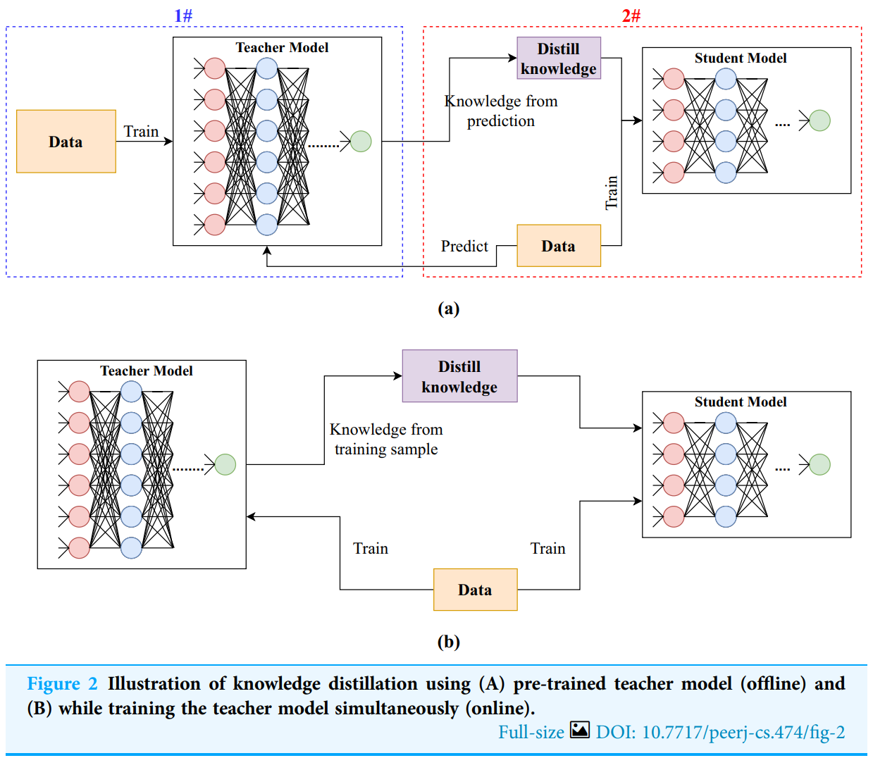
For details on the different methods, see Distilling the Knowledge in a Neural Network, Google, Knowledge distillation in deep learning and its applications, and Knowledge Distillation: A Survey.
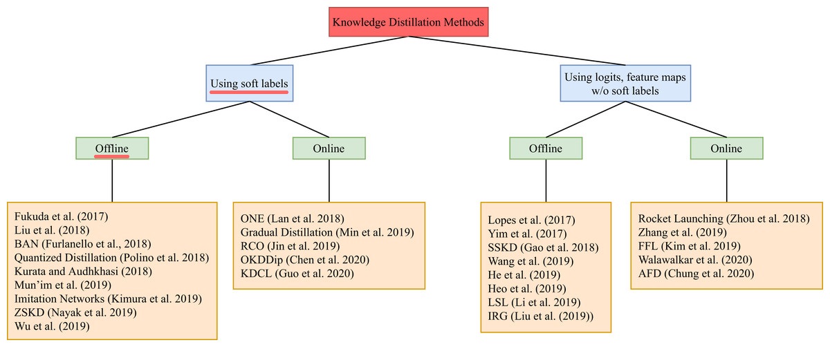
An illustration of the different categories of knowledge distillation methods, and of the branches within each category. In this section, we implement offline distillation using soft labels, underlined in red in the picture. Adapted from Knowledge distillation in deep learning and its applications.
Implementing offline distillation with soft labels
Our teacher is the pre-trained GPTlite, and our student is a smaller GPTlite with fewer layers and a smaller embedding. The teacher is frozen: it runs in evaluation mode (no dropout), and its forward pass runs inside torch.no_grad(), so that no computation graph or gradients are created for it. At every training step, both models process the same batch, and the student learns to match the teacher’s output distribution at every position of the sequence. We compute the teacher’s soft labels on the fly instead of storing them on disk: storing them takes batch size × sequence length × vocabulary size values per batch, and only pays off when the teacher is too large to run next to the student (in that case, one usually stores only the top-k logits, together with the inputs they belong to).
The loss the Kullback-Leibler (KL) divergence between the teacher’s distribution \(p\) and the student’s distribution \(q\):
\[\begin{equation} \begin{split} D_{KL}(p \parallel q) & = H(p,q) - H(p) \\ & = - \sum_i p_i \log (q_i) + \sum_i p_i \log (p_i) \\ & = \sum_i p_i \log \frac{p_i}{q_i} \end{split} \end{equation}\]where \(H(p,q)\) is the cross entropy and \(H(p)\) the entropy of the teacher’s distribution. Since \(H(p)\) does not depend on the student, minimizing the KL divergence is equivalent to minimizing the cross entropy. The loss values differ, though: the KL divergence is zero when both distributions match, while the cross entropy equals the entropy of the target. This is why the cross entropy is the usual loss for hard labels, whose entropy is zero, and the KL divergence is used to compare two distributions. In PyTorch, F.kl_div expects the student’s log-probabilities as input. We also pass the teacher’s distribution as log-probabilities (log_target=True), which the documentation recommends to avoid numerical issues. We flatten the logits to shape (batch × sequence length, vocabulary size) and use reduction='batchmean', so that the loss is the mean KL divergence per token.
The temperature \(t\) controls how soft the distributions are. For logits \(z\), the softened output is:
\[y_i (x \mid t) = \frac{ \exp\frac{z_i(x)}{t} }{ \sum_j \, \exp\frac{z_j(x)}{t} }\]A temperature above 1 flattens the distribution and reveals the relative probabilities of the unlikely tokens, which carry mot of the extra information. Since the gradients of the softened loss scale with \(1/t^2\), we multiply the loss by \(t^2\), as proposed by Hinton et al., so that the size of the gradients does not depend on the temperature. A common variant adds the regular cross entropy with the ground-truth labels, weighted by a factor \(\alpha\). There are also claims that the mean squared error between logits works better than the KL divergence (Kim et al.). For LLMs, recent methods also train the student on sequences it generated itself, scored by the teacher (on-policy distillation), which removes the mismatch between the sequences seen in training and in generation.
The following code implements the distillation of GPTlite into a smaller student. The full code is in main_distillation.py:
Show code
def distillation_loss(logits_student, logits_teacher, temperature):
  """ KL divergence between the softened teacher and student distributions, averaged per token, and
      scaled by temperature^2 so that the size of the gradients does not depend on the temperature """
  vocab_size = logits_student.size(-1)
  log_softmax_student = F.log_softmax(logits_student.reshape(-1, vocab_size)/temperature, dim=-1)   #log softmax of student model
  log_softmax_teacher = F.log_softmax(logits_teacher.reshape(-1, vocab_size)/temperature, dim=-1)   #log softmax of teacher model
  return F.kl_div(log_softmax_student, log_softmax_teacher, log_target=True, reduction='batchmean') * (temperature ** 2)

# the teacher: the pre-trained GPTlite, frozen in evaluation mode
n_layers, d_model, n_heads, d_head, batch_size, lr, seqlen, dropout_p = get_gptlite_model_parameters()
model_teacher = GPTlite(vocab_size, d_model, n_heads, d_head, n_layers, dropout_p, seqlen).to(device).eval()
model_teacher.load_state_dict(torch.load(GPTLITE_CKPT_PATH, map_location=device))

# the student: a smaller GPTlite
n_layers, d_model, n_heads, d_head, batch_size, lr, seqlen, dropout_p = get_gptlite_distilled_model_parameters()
model_student = GPTlite(vocab_size, d_model, n_heads, d_head, n_layers, dropout_p, seqlen).to(device)
optimizer = torch.optim.Adam(model_student.parameters(), lr=lr)

for step in range(1, train_iters+1):
  model_student.train()
  idx, _ = get_batch(train_data, batch_size=batch_size, seqlen=seqlen)   #get a batch of training data
  idx = idx.to(device) #move data to GPU
  logits_student = model_student(idx)   #forward pass
  with torch.no_grad():
    logits_teacher = model_teacher(idx)   #forward pass of the frozen teacher, without gradients
  loss = distillation_loss(logits_student, logits_teacher, temperature)  #compute KL divergence loss
  loss.backward()   #backward pass
  torch.nn.utils.clip_grad_norm_(model_student.parameters(), max_norm=1.0) # gradient clipping to avoid exploding gradients
  optimizer.step()   #update parameters
  optimizer.zero_grad(set_to_none=True)  #sets to None instead of 0, to save memory
The student is useful on its own, as a faster model, and as the draft model for speculative decoding (see part 2).
Pruning
Pruning removes parts of a trained model. It is a hard problem, for three reasons: we must decide what to remove without trying every option; the parts of a network are coupled, so removing one forces changes elsewhere; and removing anything hurts accuracy, which must then be recovered. A fourth difficulty is turning the removal into actual speed.
What can be removed. Unstructured pruning removes individual weights by setting them to zero. Structured pruning removes whole structures, which shrinks the weight matrices. In GPTlite, a linear layer nn.Linear(d_in, d_out) stores a weight matrix of shape d_out × d_in, so:
- removing MLP neuron \(j\) removes row \(j\) (and bias \(j\)) of the first MLP layer, and column \(j\) of the second;
- remving attention head \(h\) removes its \(d_\text{head}\) rows from the query, key and value projections, and the corresponding \(d_\text{head}\) columns of the output projection;
- removing embedding channel \(c\) removes column \(c\) of the token and position embeddings, entry \(c\) of every LayerNorm, column \(c\) of every matrix that reads from the residual stream (query, key and value projections, first MLP layer and final output layer), and row \(c\) (and bias \(c\)) of every matrix that writes to it (attention output projection and second MLP layer). Every layer changes, which makes this the hardest and most impactful dimension;
- removing a transformer block deletes it entirely; thanks to the residual connections, the shapes of the other blocks stay valid.
Unstructured sparsity needs special hardware. A weight matrix with 50% of zeros scattered at random is still multiplied as a dense matrix by GPUs, so it saves no time, and saves memory only with a sparse storage format. The exception is NVIDIA’s 2:4 semi-structured sparsity (Mishra et al.): in every group of 4 consecutive weights, 2 are zero, and the sparse tensor cores of Ampere and newer GPUs skip them, doubling the peak throughput of those matrix multiplications. The end-to-end speedups are smaller, since attention, memory traffic and the other operations are not accelerated.
How to decide what to remove. Pruning methods estimate the importance of each weight or structure, usually on a small calibration dataset:
- magnitude: small weights matter less (simple, but crude);
- activations: a neuron, head or channel whose activations are small on average contributes little (used by Minitron, below);
- weights times activations: Wanda scores each weight by \(\lvert W_{ij} \rvert \cdot \lVert X_j \rVert_2\), its magnitude times the norm of its input feature, and prunes without any retraining;
- gradients: the first-order Taylor expansion \(\lvert w \cdot \partial L / \partial w \rvert\) estimates how much the loss increases when \(w\) is removed (LLM-Pruner, which also groups coupled structures and removes them together);
- second-order information: SparseGPT prunes and updates the remaining weights to compensate, one column at a time, using the inverse Hessian (the same idea as GPTQ). It prunes 175B-parameter models to 50-60% unstructured sparsity, or to 2:4 sparsity, in one shot;
- layer redundancy: ShortGPT removes the blocks whose output is most similar to their input (by cosine similarity), since they change the hidden state the least;
- learned masks: Sheared-LLaMA learns which heads, neurons, channels and layers to keep to reach a target architecture.
The Minitron recipe. NVIDIA’s Minitron combines structured pruning with distillation:
- compute the importance of heads, MLP neurons and embedding channels from their activations, and the importance of each layer from how much removing it hurts, on a small calibration set of about a thousand samples;
- prune the model to the target architecture;
- retrain the pruned model by distilling from the original one (the KL divergence on the logits, from the previous section), using a few percent of the original training tokens;
- repeat for smaller sizes.
Deriving 8B and 4B models from a 15B one this way required up to 40 times fewer training tokens than training them from scratch, and gave better accuracy. A follow-up on Llama 3.1 8B found that width pruning (heads, neurons and channels) preserves more accuracy, while depth pruning (whole blocks) gives larger speedups. The key insight is that a pruned teacher is a much better starting point for the student than a random initialization.
We apply this recipe to GPTlite, removing half of the attention heads and MLP neurons of every block in two ways: in one shot, followed by distillation, and iteratively, removing 10% at a time and distilling after each step, with the same total number of distillation steps. As a baseline, we distill into the same small architecture from a random initialization.
The following code implements the importance of heads and neurons, the structured pruning and the experiment. The full code is in main_pruning.py:
Show code
def compute_importance(model, data, n_batches, batch_size, seqlen):
  """ Importance of every attention head (norm of its output) and every MLP neuron (absolute value of its
      ReLU output), summed over a calibration set """
  heads = [torch.zeros(block.mha.n_heads, device=device) for block in model.blocks]
  neurons = [torch.zeros(block.ffwd.net[0].out_features, device=device) for block in model.blocks]
  def head_hook(i, H, D):  # the input of the output projection concatenates the outputs of all heads
    def hook(module, inputs):
      heads[i] += inputs[0].reshape(-1, H, D).norm(dim=-1).sum(dim=0)
    return hook
  def neuron_hook(i):  # the output of the ReLU holds the activations of the MLP neurons
    def hook(module, inputs, output):
      neurons[i] += output.reshape(-1, output.size(-1)).abs().sum(dim=0)
    return hook
  hooks = []
  for i, block in enumerate(model.blocks):
    hooks.append(block.mha.out_proj.register_forward_pre_hook(head_hook(i, block.mha.n_heads, block.mha.d_head)))
    hooks.append(block.ffwd.net[1].register_forward_hook(neuron_hook(i)))
  for _ in range(n_batches):
    x, _ = get_batch(data, batch_size=batch_size, seqlen=seqlen)
    model(x.to(device))
  for hook in hooks:
    hook.remove()
  return heads, neurons

def prune(model, heads, neurons, n_heads, n_neurons):
  """ Keeps the n_heads most important heads and the n_neurons most important MLP neurons of every block """
  for block, head_importance, neuron_importance in zip(model.blocks, heads, neurons):
    mha, D = block.mha, block.mha.d_head
    keep_heads = head_importance.topk(n_heads).indices.sort().values
    rows = (keep_heads[:, None] * D + torch.arange(D, device=device)).flatten()  # the d_head rows of each kept head
    mha.query_proj = prune_linear(mha.query_proj, rows=rows)
    mha.key_proj = prune_linear(mha.key_proj, rows=rows)
    mha.value_proj = prune_linear(mha.value_proj, rows=rows)
    mha.out_proj = prune_linear(mha.out_proj, columns=rows)
    mha.n_heads = n_heads
    keep_neurons = neuron_importance.topk(n_neurons).indices.sort().values
    block.ffwd.net[0] = prune_linear(block.ffwd.net[0], rows=keep_neurons)     # first MLP layer: one row per neuron
    block.ffwd.net[2] = prune_linear(block.ffwd.net[2], columns=keep_neurons)  # second MLP layer: one column per neuron
  return model

# the experiment: one-shot and iterative pruning, followed by distillation from the original model (teacher)
model = prune(copy.deepcopy(teacher), *importance(teacher), *target_size(keep_ratios[-1]))
distill(model, teacher, train_data, distill_iters, lr, batch_size, seqlen)

model = copy.deepcopy(teacher)
for ratio in keep_ratios:
  prune(model, *importance(model), *target_size(ratio))
  distill(model, teacher, train_data, distill_iters // len(keep_ratios), lr, batch_size, seqlen)
What’s next
In the second part of this series, we generate several tokens per forward pass with speculative decoding and multi-token prediction, use fewer bits per value with quantization, remove the overheads around the math with kernel fusion and compilers, and look at architectures built for fast inference.