The Leaky Integrate-and-Fire Neuron Model and The Brunel Network
The Leaky Integrate-and-Fire neuron model (IF, first described in 1907 by Louis Lapicque) simplifies neurons complexity and assumes the neuron structure to be a single leaky compartment (point neuron model) with a membrane described by an RC circuit, as:
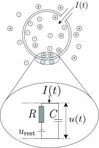
source: Neuronal Dynamics, Gerstner et al., Cambridge University Press
The main formulation of its electrical activity is given by the current equation, with the following terms:
- The current in the capacitor \(C\) is given by \(I_c = \frac{dQ}{dt} = \frac{d CV}{dt} = C \frac{dV}{dt}\)i, for charge \(Q\) and capacitance \(C\);
- The current in the resistance \(R\) is given by Ohm’s law as \(I_R = V/R\), for voltage \(V\) and resistance \(R\);
The law of conservation of energy states that the total energy of an isolated system remains constant. Thus the sum of all currents from the capacitor \(I_C\), resistance \(I_R\) and all remaining currents \(I\) must be zero. Equivalently:
\[C \frac{dV}{dt}(t) = -\frac{V(t)}{R} + I(t)\]It is common to multiply all terms by \(R\), in order to expose the time constant \(\tau = R C\). This a very important metric in the analysis of the behaviour of models, as it tells how fast are the dynamics of the neuron. The formulation becomes then:
\[\tau \frac{dV}{dt}(t) = -V(t) + RI(t) \label{equation_diff}\]We add the external currents (such as synaptic activity) to \(I(t)\). Im practice the network contribution \(RI(t)\) is described by the sum of all currents delivered from any neuron \(j\) to a given neuron \(i\) throughout time and is described as :
\[RI(t)_i = \tau \sum_{j} J_{ij} \sum_{t^\prime} \delta (t-t^\prime _{j} -D) \label{equation_current}\]where \(J_{ij}\) is the postsynaptic potential (PSP) amplitude, \(\delta (t)\) the dirac function, \(t^\prime _{j}\) the spiking time of pre-synaptic neuron \(j\) at time \(t^\prime\) and \(D\) the transmission delay. For simplicity we represent \(V(t)\) as \(V_t\).
We consider that the neuron is able to steeply rise its potential when there is an input of current, thus discarding the exponential charge of the capacitance. On the other hand, the discharge follows an exponential decay with the time constant \(\tau\).
To simulate the Action Potential (or spike) of biological neurons, we assume that each neuron has a certain fixed firing threshold. When the potential reaches its firing threshold, the neuron spikes (or fires), and immediately discharges its current to the a resting potential. Axonic branches of neurons are simulated by an synaptic delay that regulates the time that a spike signal takes to reach its connected post-synaptic neurons. This spike and current propagation that dictates the synaptic delay is illustrated in the following picture:
 source: Wikipedia
Afterwards, for a given refractory period, the neuron potential is constant at rest, in order to simulate the refraction of biological neurons. This may not be a very detailed simulation of neuron activity, but it is a good starting point of a simple neuron model, before we advance to more complicated models in future posts.
Resolution
We compute two different stepping methods from the analytical solution of the first order ODE. A two step algorithm:
- Calculate decay from previous step: \(V_t \leftarrow V_{t- \Delta t} exp(\frac{-dt}{\tau})\)
- Add voltage change of network current \(RI\) between \(t-\Delta t\) and \(t\): \(V_t \leftarrow V_t + RI_{(t-\Delta t, t]} / \tau\)
We can advance neurons with a fixed step or variable step interpolation.
- Fixed step interpolation assumes interpolation interval \(\Delta t\) to be constant throughout the execution.
- Variable step methods advance the neuron with the smallest \(t\) on the network, with a \(\Delta t\) computed as the minimum of the two following values:
- the time difference to the next incoming spike;
- \(t^\star + D\) where \(t^\star\) is the time of the neuron with the second smallest \(t\), i.e. the largest step that can be taken from neuron at \(t\) so that it won’t miss a spike from neuron at time \(t^\star\) (if it spikes) and \(D\) is the synaptic delay.
We can also solve the fixed and variable step interpolations numerically, instaed of using the analytical solution. This is a common practice for efficiency purposes, as the exponential and division operators required are computationally costly. The solution is not exact, but can appoximate well enough the solution when the timestep \(\Delta t\) is small enough. As a simple example, we can use two approximated fixed-step Euler methods:
- Explicit Forward Euler:
- Implicit Backward Euler:
with \(\frac{dV_{t}}{dt}\) and \(RI_{(t-\Delta t, t]}\) computed from equations \ref{equation_diff} and \ref{equation_current} respectively. Note that \(RI_{(t-\Delta t, t]}\) is divided by \(\Delta t\) so that it is expressed in voltage per time-unit instead of per timestep.
For the sake of comparison, we illustrate below the potential over time of a given neuron in a network, for the aforementioned methods on a \(100ms\) simulation of a (Brunel) network of \(10000\) neurons and default neuron parameters. Results are given for the Implicit and Explicit Euler methods with \(\Delta t = 0.1ms\), and for the analytical solution solved with fixed (\(\Delta t=0.1ms\)) and variable timestepping:
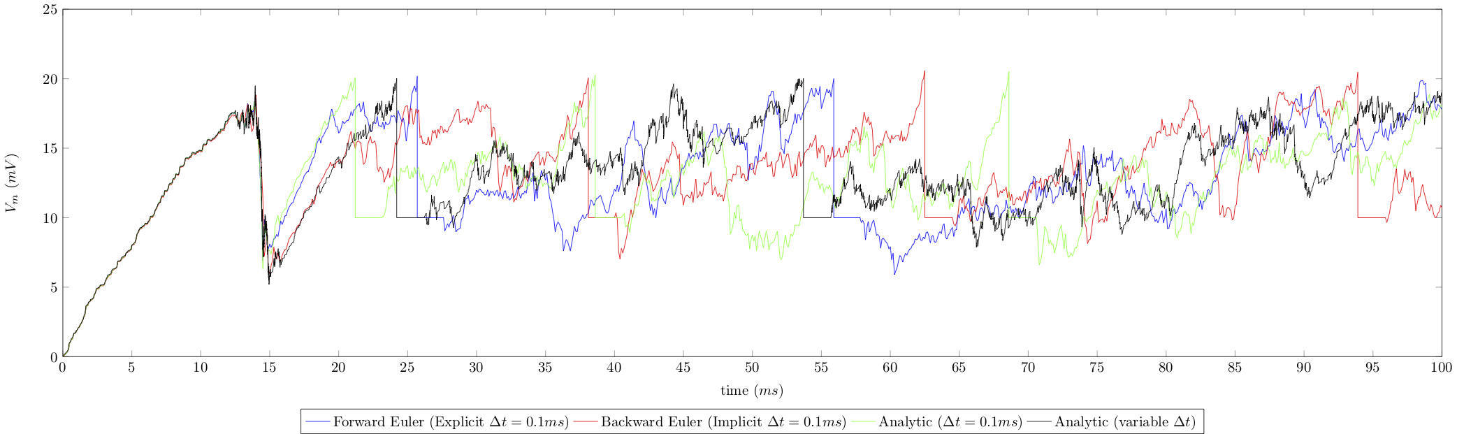
Note the vertical straight lines that refer to voltage reset after a spike, and the horizontal straight lines referring to the regractory period after firing.
Brunel Network
We’ve just mentioned network activity in the previous section. Indeed, a neuron without any kind of stimulus (either electric current injection or synaptic currents) will remain always at rest.
The most common model of network activity is called The Brunel Network Model (Dynamics of Sparsely Connected Networks of Excitatory and Inhibitory Spiking Neurons, Brunel et al., Journal Comp. Neuroscience, pdf). It is of very high relevance as it is a good estimation of network dynamics. The model proposes a network of 10000 simulated LIF neurons (80% excitatory, 20% inhibitory), with external stimuli provided by two networks of excitatory and inhibitory neurons, respectively. Excitatory means that the PSP is positive. The converse holds for inhibitory. The external networks of neurons are not stimulated, therefore its spiking is generated by a poisson random generator (PG). The diagram is the following:

source: Brunel 2000
The tricky part here is to define the parameters of the network in terms of connectivity, synaptic weights, firing threshold, etc. The original paper describes them on detail, but for simplicity, we describe them in the table bellow:

source: Marc-Oliver Gewaltig, researchgate
We can now adjust the stimuli parameters in order to regulate network activity. Brunel defines a model for slow, regular and fast dynamics of the network, that obey the following average neuron spiking rate (Hz) and global oscilation frequency (Hz) of voltage trajectories:
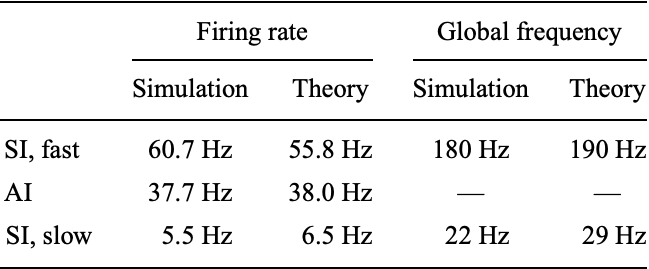
source: Brunel 2000
Notice the proximity of our simulated network model with the theoretical behaviour observed in real neurons. For that reason, although being a simple model of approximation, the Brunel Network provides a powerful tool for studying network dynamics. The model is particularly useful in very long simulations of large networks as it is computationally inexpensive compared to more detailed models such as the Hodgkin-Huxley.
Output
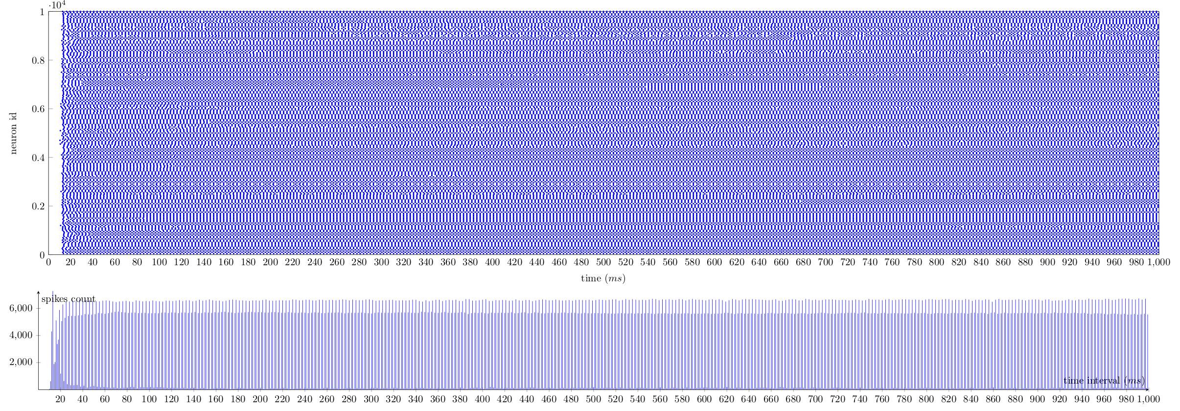
We implemented a C++ based Brunel network model of LIF neurons and injected the appropriate stimuli to recreate the original paper. The outputs match the theoretical model, in terms of spike rate and trajectory oscilation frequency. Results are presented as a time line (left-to-right) of neuron spike times (a.k.a. spike trace, on the top) and the number of neurons that spike at a given instant (bottom). Enjoy.
Slow dynamics:

Regular dynamics:

Fast dynamics:
Other resources
- For a thorough explanation of the Leaky Integrate-And-Fire Model, check the relevant section in the online copy of the Neuronal Dynamics Book from Wulfram Gerster at EPFL.
- For a
Pythonimplementation of a Brunel network using the NEST simulator, check NEST by Example: An Introduction to the Neural Simulation Tool NEST, Marc Oliver, Springer Link - For the
C++code for this exercise, download lif-brunel.tar.gz. For better code understanding, the diagram of classes is presented in diagram_class.png.