Distributed Mixture-of-Experts and Expert Parallelism
Details of GPT-4 have been the subject of widespread speculation and reporting, including a widely shared leak report that mentions the possible use of Mixture-of-Experts (MoEs): 16 experts of ~110B parameters each (≈1.8T total parameters). In practice, MoEs are attractive because they can increase model capacity per FLOP: you activate only a small subset of experts per token, which can improve scaling, efficiency, and quality compared to similarly expensive dense models.
So in this post, we will discuss MoEs development from early days, and provide implementations of MoEs on single and multiple nodes, using the PyTorch distributed API. We will discuss key concepts such as routing, sparsity, load imbalance (and corresponding loss terms), parallelism, expert capacity, numerical instabilities, overfitting and finetuning.
Early days: small MoEs as a weighted sum of expert outputs
In 1991, the papers Adaptive Mixture of Local Experts and Task Decomposition Through Competition in a Modular Connectionist Architecture introduced some of the earliest architectures similar to what we call nowadays an MoE.
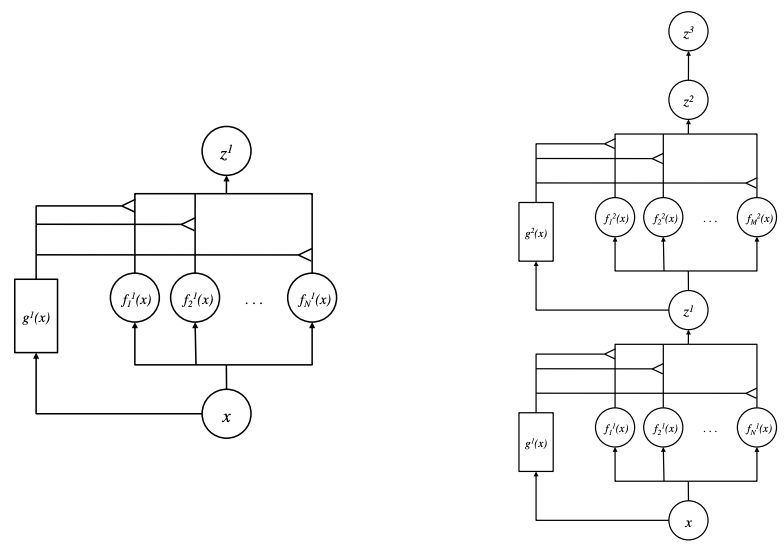
Left: a Mixture of Experts. Right: a Deep Mixture of Experts (with 2 layers).
Source: Learning Factored Representations in a Deep Mixture of Experts
The MoE was defined as a set of independent experts (feed-forward networks, \(f_i(x)\) in the picture) alongside a gating network (also a feed-forward network, \(g(x)\)). All the experts and the gating network receive the same input \(x\). The gating network outputs a distribution of each expert’s relevance/importance for the given input and can be defined in its simplest form as \(g(x) = \mathrm{Softmax}(x \cdot W_g)\), where \(W_g\) is an (optional) learnable transformation. Finally, the output of the system (\(z\)) is the sum of the outputs of all experts weighted by the output of the gating network.
The implementation of a MoE module is straightforward, and you can find the full code with running examples in the moe.py file in the supporting repository:
class MoE(nn.Module):

  def __init__(self, input_size, output_size, num_experts, dropout=0.1):
    super().__init__()
    self.router = Router(input_size, num_experts, dropout=dropout)
    self.experts = nn.ModuleList([
      FeedForward(input_size, output_size, dropout=dropout) for _ in range(num_experts) ])

  def forward(self, x):
    probs = self.router(x)
    outputs = torch.stack([ expert(x) for expert in self.experts ], dim=-2) # B*T*Experts*C
    weighted_outputs = outputs * probs.unsqueeze(-1) # B*T*E*C x B*T*E*1 -> B*T*E*C
    weighted_sum = weighted_outputs.sum(dim=-2) # sum over experts: B*T*E*C -> B*T*C
    return weighted_sum, probs, outputs
A major difference between the two 1991 approaches is the loss function used. One can pick an error function \(E = \| d - \sum_i p_i \, o_i \| ^2\), where \(o_i\) is the output vector of expert \(i\), \(p_i\) is the router’s probability for expert \(i\), and \(d\) is the correct label for the input. The other argues that this form can lead to starvation of experts (some experts are never assigned any importance) and overpowering (one expert gets most of the probability mass). It suggests instead the error function \(E = \sum_i p_i \| d - o_i \| ^2\) (and variants based on negative log-likelihood).
def loss_per_token_Adaptive_Mixture_1991(probs, outputs, labels):
  """
  outputs: B*T*E*Classes
  probs:   B*T*E
  labels:  B*T (class ids)
  returns: B*T (loss per token)
  """
  one_hot = torch.nn.functional.one_hot(labels, num_classes=outputs.shape[-1]).to(outputs.dtype) # B*T*Classes
  # per-token MSE for each expert: B*T*E
  mse = (one_hot.unsqueeze(-2) - outputs).square().mean(dim=-1)  # mean over Classes
  return (mse * probs).sum(dim=-1)  # weighted sum over experts -> B*T
An important observation related to the behaviour of MoEs, where the authors observed that
the learning procedure divides up a vowel discrimination task into appropriate subtasks, each of which can be solved by a very simple expert network.
Deep Mixture of Experts
With the surge of deep neural networks, Learning Factored Representations in a Deep Mixture of Experts (2014) extended “Mixture of Experts” to a stacked model (“Deep Mixture of Experts”) with multiple sets of gating and experts.
This deep MoE model can be coded simply by stacking several MoE layers (also available in moe.py):
class MoE_deep(nn.Module):
  def __init__(self, input_size, output_size, num_experts, depth=2, dropout=0.1):
    super().__init__()
    self.stack = nn.ModuleList(
      [MoE(input_size, input_size,  num_experts, dropout) for _ in range(depth-1)] +
      [MoE(input_size, output_size, num_experts, dropout)]
    )

  def forward(self, x):
    # each MoE returns (weighted_sum, probs, outputs); we feed forward only the weighted_sum
    for layer in self.stack:
      x, _, _ = layer(x)
    return x
During training, as before, the authors noticed that training led to a degenerate local minimum: “experts at each layer that perform best for the first few examples end up overpowering the remaining experts”, because as they are better initially, then end up being picked more by the gates. This was overcome by capping (max clipping) the assignments to a maximum value, and re-normalizing across all (post max-clipping) gating probabilities. This cap value is then removed in a second training stage.
The benchmark compared a single MoE, a two-level MoE, a two-layer MoE where the information between layers is the concatenation of all layer-1 experts (instead of the weighted sum of outputs), and a regular feed-forward network with a similar number of parameters. Results showed that, “In most cases, the deeply stacked experts perform between the single and concatenated experts baselines on the training set, as expected. However, the deep models often suffer from overfitting: the mixture’s error on the test set is worse than that of the single expert for two of the four model sizes. Encouragingly, the DMoE performs almost as well as a fully-connected network (DNN) with the same number of parameters, even though this network imposes fewer constraints on its structure”.
An important result emphasizes the relevance of stacking MoEs into a deep model:
we find that the Deep Mixture of Experts automatically learns to develop location-dependent (“where”) experts at the first layer, and class-specific (“what”) experts at the second layer.
And this led to the follow up work that explored having the gating being used not only to weight the sum of output of experts, but as well as a router of the input to individual experts, as we will see in the following section.
Sparsely-Gated Mixture of Experts
The previous MoE implementations had a big drawback: all experts process all inputs, leading to high training costs, even when there’s little relevance of some experts for some inputs. This led to conditional computation / sparsity, where only a subset of experts are picked per input. In practice, the distribution output by the gating mechanism is now used to pick only the highest-relevance experts for each token and route the token only to those top-\(k\) experts, effectively working as a routing mechanism. \(k\) is a hyper-parameter that drives the trade-off between computation and expertise.
In practice, the MoE selects for each token in the text a possibly different combination of experts. When \(g_i(x)=0\) for a given expert \(i\), then \(f_i(x)\) is not computed. Note that, by picking only top-\(k\) experts per token, one can increase the number of experts without incurring proportional computational overhead, which is the key MoE scaling property.
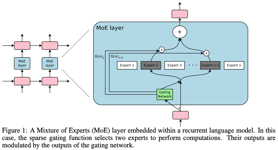
Towards better scaling, the 2017 paper Outrageously Large Neural Networks: The Sparsely-Gated Mixture-of-Experts Layer presented a recurrent (LSTM-based) language model where the feed-forward subnetwork was replaced with an MoE structure. The objective was to do text processing (and translation) with thousands of experts, totalling 137B parameters:
Processing and batching
The MoE is called once for each position in the text, selecting a potentially different combination of experts at each position. Because this can lead to very small effective per-expert batches (the “shrinking batch problem”), they suggest using a very large global batch size to overcome it.
Parallelism and Hierarchical MoEs
To enable parallelism, the authors implement data and model parallelism: they “distribute the standard layers of the model and the gating network according to conventional data-parallel schemes, but keep only one shared copy of each expert” (i.e., experts are sharded rather than replicated).
Although they tested thousands of experts, if the number of experts is very large, they also reduce the branching factor by using a two-level hierarchical MoE. A hierarchical MoE is a structure where a primary gating network chooses a sparse weighted combination of experts, and each selected expert is itself an MoE with its own gating network. In the case of their hierarchical MoE, the primary gating network employs data parallelism, and the secondary MoEs employ model parallelism; each secondary MoE resides on one device.
Improvements specific to language models: convolutionality
When applied to a language task, they take advantage of convolutionality where each expert is applied in the same way to each time step. This allows applying the MoE to all the time steps together as one big batch, increasing effective utilization.
Gating and Sparsity
Instead of the typical softmax gating \(G(x) = \mathrm{softmax}(x \cdot W_g)\), the paper proposes sparsity via noisy top-k gating, where they add tunable Gaussian noise \(H(x)\), controlled by \(W_{noise}\). To handle sparsity, non-top-\(k\) experts are set to \(-\infty\) before the softmax so their post-softmax value becomes 0:
\[G(x) = \mathrm{softmax}(\, \mathrm{KeepTopK}(\, H(x), k) \;)\] \[H(x)_i = (x \cdot W_g)_i + \mathrm{StandardNormal}() \cdot \mathrm{Softplus}((x \cdot W_{noise})_i)\]Note: \(\mathrm{Softplus}\) keeps the noise scale positive.
Importance loss
To avoid overpowering / starvation of experts, they add an additional importance loss, equal to the square of the coefficient of variation of the set of importance values:
\[L_{importance} = w_{importance} \cdot CV(\, \mathrm{Importance}(X)\,)^2\]where \(CV = \sigma/\mu\) is the ratio of standard deviation to mean. The importance of an expert is computed as the batchwise sum of the gate values for that expert, and \(w_{importance}\) is a hand-tuned scaling factor. As an example, take a batch of 4 samples \(x_i\) assigned across 5 experts \(E_j\), with the following distribution:
| \(E_1\) | \(E_2\) | \(E_3\) | \(E_4\) | \(E_5\) | |
|---|---|---|---|---|---|
| \(x_1\) | 0.1 | 0.1 | 0 | 0.8 | 0 |
| \(x_2\) | 0 | 0 | 0.2 | 0.7 | 0.1 |
| \(x_3\) | 0.1 | 0 | 0 | 0.9 | 0 |
| \(x_4\) | 0 | 0 | 0 | 1 | 0 |
| Importance (sum) | 0.2 | 0.1 | 0.2 | 3.4 | 0.1 |
In this example, the mean of the importance is \(\mu = 0.8\) and the population standard deviation is \(\sigma \approx 1.30\), thus \(CV \approx 1.62\). If experts were assigned similar importance, the variance would be smaller and the CV also smaller, thus reducing the importance loss.
Load loss
The previous importance loss tries to balance overall importance across experts, but experts may still receive different numbers of tokens. This may lead to memory and compute imbalance on distributed hardware, and to having experts that are undertrained. To solve this, a second load loss \(L_{load}\) is introduced that encourages experts to receive a similar amount of training samples. However, the hard token count is a constant and cannot be backpropagated, so instead they use a smooth operator \(\mathrm{Load}(X)\) that can be backpropagated:
\[L_{load}(X)_i = \sum_{x \in X} P(x,i)\]where \(P(x,i) = Pr(H(x)_i) \gt kth\_excluding(H(x), k, i)\) denotes the probability that \(G(x)_i\) is non-zero, given a new random choice of noise on element \(i\), but keeping the already-sampled choices of noise on the other elements (see Appendix A for details). Note that \(G(x)_i\) is non-zero iff \(H(x)_i\) is greater than the \(k\)-th greatest element of \(H(x)\).
Results
The experiments fixed a compute budget and compared a baseline model with several configurations of MoE, including a hierarchical MoE, on several language tasks. Results show that:
- MoE models beat baseline LSTM models, with hierarchical MoE beating non-hierarchical (with higher parameter count but similar compute per example).
- The perplexity improved significantly by increasing data size (from 10B to 100B Word Google News Corpus). In a machine translation task, on the Google Production dataset, the model achieved 1.01 higher test BLEU score even after training for only one sixth of the time.
- In terms of scalability, the results claim to obtain “greater than 1000x improvements in model capacity with only minor losses in computational efficiency”.
- Learning to route does not work without the ability to compare at least two experts (stability issues), motivating top-2 routing in that work.
Finally, they look at input-to-expert assignments that demonstrate that different experts specialize on different tasks based on syntax and semantics (Appendix E table 9):
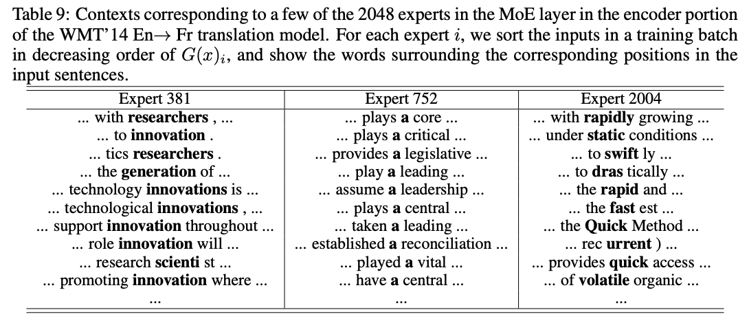
Due to lack of time, I am not providing an implementation, but for the record, a simple python implementation of this model is available in this repo.
Conditional Computing for improved scaling
In 2020, GShard: Scaling Giant Models with Conditional Computation and Automatic Sharding explored the scaling of Transformer-based sparsely-gated MoEs up to 600B parameters on a sequence-to-sequence (machine translation) task. They claim sub-linear compute growth with model capacity and essentially constant compilation time on large TPU pods.
It reutilizes some efficiency techniques from the previous paper. The first is the position-wise Sparsely-Gated MoEs for language tasks (section 2.2), delivering sub-linear scaling. The second is parallel partitioning as a combination of data-parallel and sharding: (1) “the attention layer is parallelized by splitting along the batch dimension and replicating its weights to all devices”; and (2) “experts in the MoE layer are infeasible to be replicated in all the devices due to its sheer size and the only viable strategy is to shard experts into many devices”.
The main improvements come from compile optimizations with Accelerated Linear Algebra (XLA) and user-flagged parallelism of tensors, as described next.
Compiler and SPMD optimizations
GShard allows for a module that separates model description from the parallel partitioning, consisting “of a set of simple APIs for annotations, and a compiler extension in XLA for automatic parallelization.” In practice, GShard “requires the user to annotate a few critical tensors (in the model) with partitioning policies”. This allows developers to write the module and the runtime will automatically partition modules across compute units. This enables a compiler technique for Single Program Multiple Data (SPMD) transformation that generates a single program to run on all devices, keeping compilation time largely independent of device count (see Figure 2 in the paper).
The XLA SPMD partitioner for GShard “automatically partitions a computation graph based on sharding annotations. Sharding annotations inform the compiler about how each tensor should be distributed across devices”.
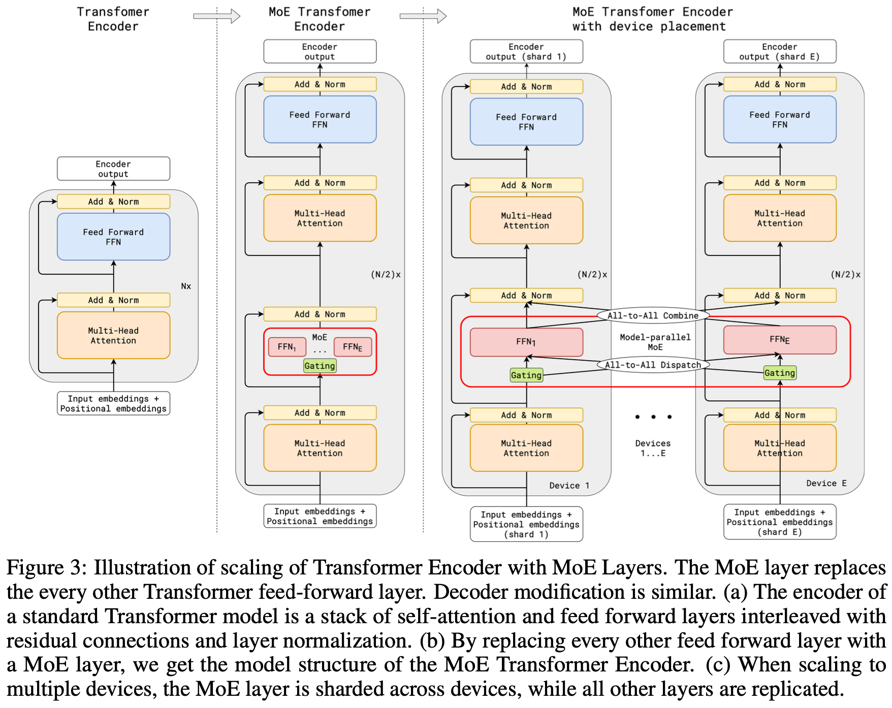
Model architecture
The model tested was a Transformer-based stack of encoder and decoder layers. Each Transformer block (self-attention, feed-forward and, on the decoder’s case, cross-attention) was converted into a conditional computation module by replacing the feed-forward layer in every second block with a MoE layer (with top-2 gating) in both the encoder and the decoder.
Random routing and expert capacity
The paper introduces the concept of expert capacity, which is the maximum number of tokens that can be assigned to an expert per iteration, set to be of order \(O(N/E)\) for \(N\) tokens and \(E\) experts. Tokens assigned to an expert at maximum capacity are considered overflow tokens and are passed to the next layer via a residual connection.
The routing mechanism applies random routing where, in the top-2 setup, the top expert always receives a token, but the second expert has a probability (related to its routing weight) of also receiving the token. I.e. it’s effectively a top-1 or top-2 setup depending on whether the 2nd expert is picked. The rationale is that if the 2nd expert has very small routing weight, its contribution is close to insignificant, so the token only needs to be passed to the first expert, reducing compute and overflow.
Auxiliary loss and load balancing
The total loss is described as \(L = l_{nll} + k \cdot l_{aux}\), where \(l_{nll}\) is the negative log-likelihood loss, \(k\) is a constant, and \(l_{aux}\) is an auxiliary loss to help avoid a few experts stealing most tokens early in training. This auxiliary loss is formulated as
\[l_{aux} = \frac{1}{E} \sum^E_{e=1} \frac{c_e}{S} \, m_e\]where the term \(c_e/S\) represents the fraction of input routed to each expert and \(m_e\) is the mean gates per expert (note that \(m_e\) is added because \(c_e/S\) is a constant and is not differentiable).
Switch Transformers
A big issue with large MoEs is training instability. With that in mind, the 2021 paper Switch Transformers: Scaling to Trillion Parameter Models with Simple and Efficient Sparsity tackled that problem by simplifying the routing algorithm and improving model specifications, delivering the first large MoE models able to be trained on bfloat16.
The benefit of scale was exhaustively studied in Scaling Laws for Neural Language Models which uncovered powerlaw scaling with model size, data set size and computational budget, [and] advocates training large models on relatively small amounts of data as the computationally optimal approach. Heeding these results, we investigate a fourth axis: increase the parameter count while keeping the floating point operations (FLOPs) per example constant.
In order to achieve scaling, the sparsely activated layers split unique weights across devices. As in GShard, the authors replace the feed-forward network with an MoE. In Switch Transformers, they use Switch routing: each token is routed to only a single expert (top-1). The claim is that this simplification preserves model quality while reducing routing computation and improving stability.
![]()
Expert Capacity
They introduce the concept of expert capacity factor, which is the number of tokens that each expert computes, computed as tokens-per-expert times a capacity factor. If this capacity factor is exceeded (i.e. if the router sends too many inputs to a given expert), then extra tokens do not have computation associated with them and are instead passed to the next layer via a residual connection.
![]()
Related to the expert capacity hyperparameter:
Increasing the capacity factor increases the quality but also increases the communication overhead and the memory in the activations. A recommended initial setup is to use an MoE with a top-2 routing with 1.25 capacity factor, with one expert per core. At evaluation time, the capacity factor can be changed to reduce compute.
Load Balancing loss
The loss function includes a simplified version of the auxiliary loss from Outrageously Large Neural Networks: The Sparsely-Gated Mixture-of-Experts Layer, which originally had separate load-balancing and importance-weighting losses. This auxiliary loss is added to the total model loss, for every Switch layer.
Given \(N\) experts and a batch \(B\) with \(T\) tokens, the auxiliary loss is computed as the scaled dot-product between vector \(f\) of fraction of tokens and \(P\) as the fraction of the router probability allocated to each expert, as:
\[loss = \alpha \cdot N \cdot \sum_{i=1}^{N} f_i \cdot P_i\]where \(\alpha\) is a user-picked hyper-parameter. Both \(P\) and \(f\) vectors should ideally have a uniform distribution, i.e. values \(1/N\).
Model size reduction via distillation
One of the downsides of these MoEs was the large number of parameters. However, it was observed that distillation was feasible if we want to operate on a smaller network:
Successful distillation of sparse pre-trained and specialized fine-tuned models into small dense models. We reduce the model size by up to 99% while preserving 30% of the quality gains of the large sparse teacher.
Finally, the paper includes several details on training techniques and experiments, that will be omitted for brevity. A single device implementation of Switch Transformers is available in this page.
Distributed implementation in PyTorch
The MoE workflow is a four-step algorithm, best illustrated in the MegaBlocks paper (detailed later):
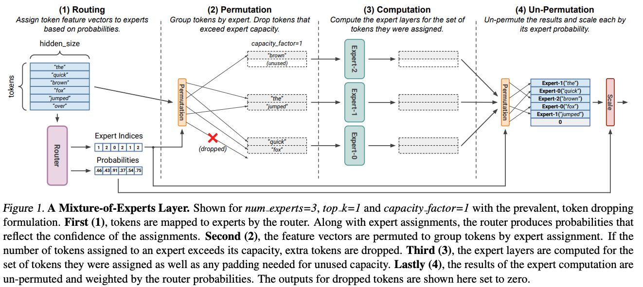
We start by defining our distributed mixture-of-experts block as MoE_dist, with a sharded router and a local expert. For the sake of simplicity, we will have a single expert per GPU, and will drop the tokens that exceed each expert’s capacity:
class MoE_dist(nn.Module):
  def __init__(self, n_embd, k=2, capacity_factor=1.25, padding_val=0, local_rank=None):
    super().__init__()
    self.capacity_factor = capacity_factor
    self.padding_val = padding_val
    self.num_experts = dist.get_world_size() # 1 expert per GPU
    self.k = k

    if local_rank is None:
      local_rank = int(os.environ.get("LOCAL_RANK", dist.get_rank()))
    device = torch.device("cuda", local_rank)

    self.router = DDP(Router(n_embd, self.num_experts).to(device), device_ids=[local_rank])
    self.expert = FeedForward(n_embd).to(device)
In here, the Router is a feed-forward network that takes as input the embedding of a token, and outputs a distribution of allocations (probabilities) over the experts. Also, we will assume there is only one expert per process, thus the process id matches the expert id, and the expert count matches the distributed network size.
The routing step computes the top-k expert assignments for each token, as expert id in topk_experts and corresponding probabilities topk_probs:
  def forward(self, x):
    # x: B*T*C
    B, T, C = x.shape
    global_rank = dist.get_rank()
    probs = self.router(x) # get assignments from router, shape B*T*n_experts
    topk_probs, topk_experts = torch.topk(probs, k=self.k, dim=-1) # B*T*k

    ids_per_expert = [ (topk_experts==expert).nonzero() for expert in range(self.num_experts) ]
    probs_per_expert = [ topk_probs[topk_experts==expert] for expert in range(self.num_experts) ]
The following permutation step selectively sends the tokens to each expert’s processor. We will use collective communication, and perform this in two steps: an all_to_all operation to exchange the amount of items to send/receive, followed by an all_to_all_single to exchange the metadata of the tokens and the token themselves (based on those counts):
    device = x.device

    # all-to-all to exchange the count of inputs to send/receive to/from each processor
    send_count = [torch.tensor([len(ids)], dtype=torch.int64, device=device) for ids in ids_per_expert]
    recv_count = [torch.tensor([0], dtype=torch.int64, device=device) for _ in ids_per_expert]
    dist.all_to_all(recv_count, send_count)
    fn_count = lambda tensor, scale=1: [x.item()*scale for x in tensor]

    # send/receive the metadata (b, t, which_topk) to/from the appropriate processors
    M = ids_per_expert[0].shape[-1] # number of columns in metadata
    send_ids = torch.cat(ids_per_expert, dim=0).to(device)
    send_ids[:,0] += global_rank*B # add processor's batch offset
    recv_ids = torch.zeros(sum(recv_count)*M, dtype=send_ids.dtype, device=device)
    dist.all_to_all_single(recv_ids, send_ids.flatten(), fn_count(recv_count,M), fn_count(send_count,M))
    recv_ids = recv_ids.view(-1, M) # reshape to M columns

    # send/receive input tokens to/from the appropriate processors
    send_toks = torch.cat([ x[ids[:,0], ids[:,1]] for ids in ids_per_expert], dim=0).to(device)
    recv_toks = torch.zeros(sum(recv_count)*C, dtype=x.dtype, device=device)
    dist.all_to_all_single(recv_toks, send_toks.flatten(), fn_count(recv_count,C), fn_count(send_count,C))
    recv_toks = recv_toks.view(-1, C) # reshape to C columns
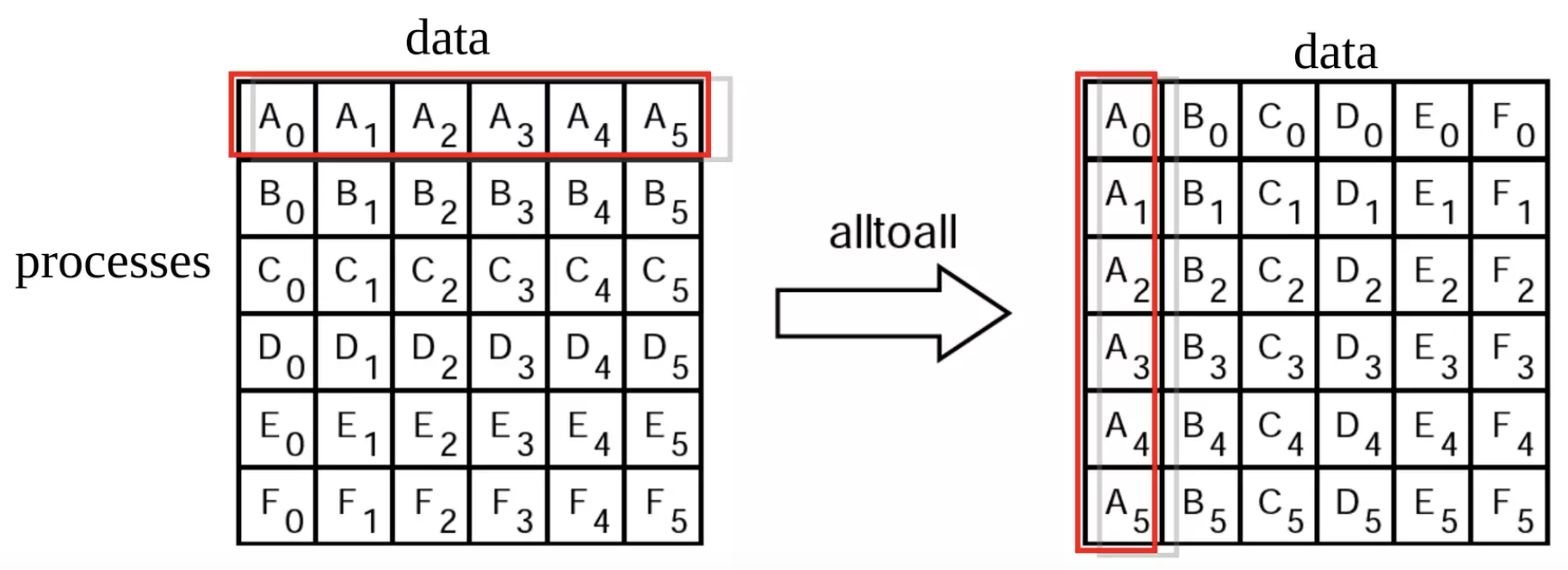
An illustration of the MPI all-to-all collective operation. When sending only 1 element per row, it is equivalent to a distributed matrix transpose - note the red row before the all-to-all (left) as a transposed column after the all-to-all (right). We use a single-element all-to-all to exchange the count of items to be sent received among processors. We then use those counts to perform a new all-to-all with variable-sized elements in the permutation step. Finally, in the un-permutation step, we perform another all-to-all that performs the converse communication, by swapping the send and receive counts and buffers.
The computation step will reshuffle the received data into a 3D batch of size Rows x Capacity x Embedding that will either crop or pad sequences to the capacity of each expert:
    # group received metadata by row id
    uniq_rows, recv_row_lens = recv_ids[:,0].unique(sorted=True, return_counts=True)
    recv_row_offsets = [0] + torch.cumsum(recv_row_lens, dim=0).tolist()
    recv_row_slice = lambda row: slice(recv_row_offsets[row], recv_row_offsets[row+1])

    # crop or pad received items PER SENTENCE to max capacity. Batch shape: Rows * Capacity * C
    capacity = int(T / self.num_experts * self.capacity_factor)
    pad_fn = lambda toks, value = self.padding_val: F.pad(toks, (0,0,0,capacity-toks.shape[0]), value=value) # pad or crop
    batch_toks = torch.stack([ pad_fn(recv_toks[recv_row_slice(i)][:capacity]) for i in range(len(uniq_rows))], dim=0).to(device)

    batch_row_len = torch.tensor([ min(recv_row_lens[r], capacity) for r in range(len(uniq_rows))], device=device)
    batch_toks = self.expert(batch_toks) # Rows * Capacity * C
The output of the expert is stored in batch_toks. The following Un-permutation step will now perform an all_to_all_single that performs the opposite communication of the permutation step. This will populate the all-to-all output buffer with the partial results of all experts.
    # scatter computed outputs back into recv_toks (only for the non-padding part)
    out_flat = torch.full_like(recv_toks, fill_value=self.padding_val)
    cursor = 0
    for r in range(len(uniq_rows)):
      n = int(batch_row_len[r].item())
      out_flat[cursor:cursor+n] = batch_toks[r, :n]
      cursor += int(recv_row_lens[r].item())

    # send back
    send_toks = torch.empty(sum(send_count)*C, dtype=x.dtype, device=device)
    dist.all_to_all_single(send_toks, out_flat.flatten(), fn_count(send_count,C), fn_count(recv_count,C))
    x = send_toks.view(-1, C)
Finally, the scale step performs a weighted sum of the top-k probabilities for each token:
    x *= torch.cat(probs_per_expert).view(-1,1) # multiply by router probabilities
    if self.k>1: # sum over k probabilities for each input
      x = torch.stack([ x[send_ids[:,-1]==kk] for kk in range(self.k)]).sum(dim=0)
    return x.view(B,T,C)
You can find the complete implementation in the Mixture-of-Experts repo.
Applying the MoE to an existing LLM
Remember that the MoE module can be used to replace the feed-forward module in existing architectures. So here we will apply it to the GPT2-based GPTlite model we built on a previous post. This is straightforward, and all we need to do is to distribute its modules in a Distributed Data Parallel fashion, except the feed-forward module in the transformer block, that we will replace by our model-parallel mixture of experts:
  # ddp function takes a torch module and distributes it in a data parallel fashion
  ddp = lambda module: DDP(module.to(device), device_ids=[local_rank])

  model = GPTlite(vocab_size) # instantiate GPTlite locally
  model.token_embedding_table = ddp(model.token_embedding_table)
  model.position_embedding_table = ddp(model.position_embedding_table)
  model.ln = ddp(model.ln)
  model.lm_head = ddp(model.lm_head)
  for b, block in enumerate(model.blocks):
    block.sa = ddp(block.sa)
    block.ln1 = ddp(block.ln1)
    block.ln2 = ddp(block.ln2)
    block.ffwd = MoE_dist(n_embd=n_embd) # replace FeedForward with a MoE (parallelism handled inside)
The rest of the training and optimization algorithm needs no changes.
Finally, note that the previous code is a bit complex if you do not come from an HPC background. If you don’t want the hassle of writing all the communication steps from scratch, you can use a library to do it for you such as DeepSpeed Mixture of Experts.
Further reading
There is plenty of research ongoing on MoEs finetuning, scaling and model variants. If you want to know more about those topics, here are some useful pointers:
2022 MegaBlocks: Efficient Sparse Training with Mixture-of-Experts
MegaBlocks is “a system for efficient Mixture-of-Experts (MoE) training on GPUs”, that addresses the model quality vs hardware efficiency tradeoff on the dynamic routing of MoE layers. In detail, the load-imbalanced computation on MoEs forces one to either (1) drop tokens from the computation or (2) waste computation and memory on padding, a parameter that is usually improved via hyperparameter tuning. However, we know that “The loss reached by the MoE models decreases significantly as expert capacity is increased, but at the cost of additional computation” and “the lowest loss is achieved by the ‘max expert capacity value’, which avoids dropping tokens through the dynamic capacity factor mechanism proposed by Adaptive mixture-of-experts at scale (2002)”. So not dropping tokens is ideal.
As a second motivation, “the sparse computation in MoEs does not map cleanly to the software primitives supported in major frameworks and libraries”. To overcome these limitations, MegaBlocks “reformulates MoE computation in terms of block-sparse operations and develop new block-sparse GPU kernels that efficiently handle the dynamism present in MoEs”. In practice, it proposes an approach of MoE routing based on sparse primitives, that matches efficiently to GPUs and never drops tokens, “ enabling end-to-end training speedups of up to 40% and 2.4× over state of the art”. This is achieved by performing block-sparse operations in the MoE layers to accommodate imbalanced assignment of tokens to experts. This is called dropless-MoEs (dMoEs) and contrasts with regular MoEs that use batched matrix multiplication instead. These dropless-MoEs kernels use blocked-CSR-COO encoding and transpose indices to enable efficient matrix products with sparse inputs.
2022 Towards Understanding Mixture of Experts in Deep Learning
Formally studies “how the MoE layer improves the performance of neural network learning and why the mixture model will not collapse into a single model”. It experiments on a 4-cluster classification vision task and claims that: (1) “cluster structure of the underlying problem and the non-linearity of the expert are pivotal to the success of MoE”; (2) there needs to be non-linearity in the experts for an MoE system to work; and (3) “the router can learn the cluster-center features, which helps divide the input complex problem into simpler linear classification sub-problems that individual experts can conquer”.
2022 GLaM: Efficient Scaling of Language Models with Mixture-of-Experts
Introduces GLaM (Generalist Language Model), a family of dense and sparse decoder-only language models, “which uses a sparsely activated mixture-of-experts architecture to scale the model capacity while also incurring substantially less training cost compared to dense variants”. GLaM has 1.2 trillion parameters (7x larger than GPT-3’s 175B) but requires 1/3 of the energy for training, and half of the computation FLOPs for inference, while “achieving better overall zero, one and few-shot performance across 29 NLP tasks” (Table 1, Figure 1).
Results were collected by training several variants of GLaM to study the behavior of MoE and dense models on the same training data (Table 4). The study highlights the that:
- “the quality of the pretrained data also plays a critical role, specifically, in the performance of downstream tasks” (section 6.2);
- sparse models scale better (section 6.3);
- “MoE models require significantly less data than dense models of comparable FLOPs to achieve similar zero, one, and few-shot performance” (section 6.4).
2022 ST-MoE: Designing Stable and Transferable Sparse Expert Models
Presents a study with experiments, results and techniques related to the stability of training and fine-tuning of very large sparse MoEs. Also introduces the router z-loss, that resolves instability issues and improves slightly the model quality, and a 269B sparse model – the Stable Transferable Mixture-of-Experts or ST-MoE-32B - that achieves state-of-the-art performance across several NLP benchmarks. The z-loss formulation is:
\[L_z(x) = \frac{1}{B} \sum_{i=1}^B \left( \log \sum_{j=1}^N e^{x_j^{(i)}} \right)\]where \(B\) is the number of tokens, \(N\) is the number of experts, and \(x \in \mathbb{R}^{B\times N}\) are the logits going into the router. The rationale behind z-loss is that it penalizes large logits into the gating network. The paper also contains a very extensive analysis of quality-stability trade-off techniques and results:
- “Sparse models often suffer from training instabilities (Figure 1) worse than those observed in standard densely-activated Transformers. […] Some architectural improvements involve more multiplications than additions or do not sum many items at once”: the paper studies GELU Gated Linear Units (GEGLU) and Root Mean Square Scale Parameters.
- Adding noise (input-jitter) and adding dropout improves stability, but leads to a significant loss of model quality (Section 3.2).
- Gradient clipping in updates (in Adafactor optimizer) improves stability, but at a high loss of quality (Section 3.3).
- Sparse expert models are sensitive to roundoff errors (eg due to lower precision representation) because they have more exponential functions due to the routers (Section 3.4).
- Sparse models are prone to overfit (Fig. 3).
- Adding dropout at 0.1 provides modest boosts while higher rates penalizes performance; and selectively increasing experts dropout increase accuracy (Fig. 4).
- Updating the non MoE parameters (while freezing others) yields an accuracy similar to updating all the parameters; and updating only the FFN parameters works a bit better (Fig 5).
- “Sparse models benefit from noisier hyperparameters including small batch sizes and high learning rates. Dense models behave nearly oppositely” (Fig. 6).
- “Sparse models are robust to dropped tokens when fine-tuning. […] dropping 10-15% of tokens can perform approximately as well as models that drop < 1%” (Table 5).
The paper provides the following 3 recommendations when designing sparse systems:
- top-2 routing with 1.25 capacity factor and at most one expert per core.
- the capacity factor can be changed during evaluation to adjust to new memory/compute requirements.
- dense layer stacking and a multiplicative bias can boost quality (Appendix C).
Related to the functioning of mixture of experts, the authors showed that encoder experts learn very shallow tasks, e.g. punctuation, nouns, etc. I.e., MoEs subdivide a problem into smaller problems that can be solved by different experts combined. The authors show this by “visualizing how tokens are routed among (encoder) experts, […] by passing a batch of tokens to the model and manually inspecting token assignment at each layer”. They observed that at each layer, at least one expert specializes in sentinel tokens (mask tokens that represent blanks to fill in); and some encoder experts exhibit clear specialization, with some experts primarily operating on punctuation, verbs, proper names, counting, etc. These are detailed in tables 13 and 15.
At the decoder level, “expert specialization is far less noticeable in the decoder”, and meaningful specialization (semantics or syntax) is not visible in decoder experts:
We hypothesize that this lack of meaningful expert specialization is caused by the distribution of target tokens induced by the span corruption objective. In particular, (a) a smaller number of tokens are routed jointly in the decoder due to longer sequence lengths in the encoder (e.g. group size is 2048 in the encoder vs 456 in the decoder in our setup) and (b) a higher proportion of tokens are sentinel tokens in the decoder. As a result, target tokens in each group typically cover a smaller semantic space (compared to the encoder), perhaps explaining the lack of expert specialization in the decoder
2022 Tutel: Adaptive Mixture-of-Experts at Scale
According to the authors, existing sparsely-gated mixture-of-experts (MoE) “suffer inefficient computation due to their static execution, namely static parallelism and pipelining, which does not adapt to the dynamic workload”. To that extent, they present Tutel, a system that delivers two main novelties: adaptive parallelism for optimal expert execution and adaptive pipelining for tackling inefficient and non-scalable dispatch/combine operations in MoE layers.
2023 Mixture-of-Experts Meets Instruction Tuning: a Winning Combination for Large Language Models
This paper claims that Instruction tuning supplemented by further finetuning on individual downstream tasks outperforms fine-tuning or instruction-tuning alone. To show that they perform single-task fine-tuning, multi-task instruction-tuning and multi-task instruction-tuning followed by single-task fine-tuning. They showed that MoEs benefit more from instruction tuning than other models and benefit more from a higher number of tasks. In practice:
in the absence of instruction tuning, MoE models fall short in performance when compared to dense models on downstream tasks. […] When supplemented with instruction tuning, MoE models exceed the performance of dense models on downstream tasks, as well as on held-out zero-shot and few-shot tasks.
2023 From sparse to soft mixture of experts
Soft MoE is a fully-differentiable sparse Transformer that rather than employing a sparse and discrete router that tries to find a good hard assignment between tokens and experts (like regular MoEs), Soft MoEs instead perform a soft assignment by mixing tokens.
In practice, it computes several weighted averages of all tokens (with weights depending on both tokens and experts) and then processes each weighted average by its corresponding expert.
It addresses the challenges of current sparse MoEs: training instability, token dropping, inability to scale the number of experts, and ineffective finetuning.
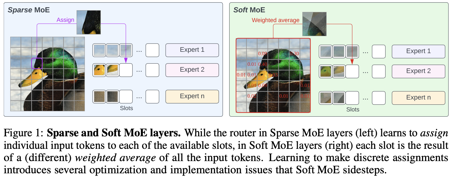
In the benchmark, Soft MoEs greatly outperforms dense Transformers (ViTs) and popular MoEs (Token Choice and Experts Choice) on a vision task, while training in a reduced time frame and delivering faster inference.
2024 Mixtral of Experts
The current state-of-art MoE model is the Mixtral 8x7B, a sparse mixture of experts, with the same architecture as Mixtral 7B except that it supports a fully dense context length of 32k tokens and the feed-forward blocks are replaced by a Mixture of 8 feed-forward network experts. Model architecture is detailed in Table 1. It performs a top-2 routing, and because tokens can be allocated to different experts, “each token has access to 47B parameters, but only uses 13B active parameters during inference”.
The formulation of the model, in section 2.1, matches the GShard architecture (except that the MoE is in every layer instead of every second), with sparse top-\(k\) MoE with gating \(G(x) = \mathrm{Softmax}(\mathrm{TopK}(x \cdot Wg))\) where \(\mathrm{TopK}(\ell)= -\infty\) for the non top-\(k\) experts. As before, “in a Transformer model, the MoE layer is applied independently per token and replaces the feed-forward (FFN) sub-block of the transformer block”. They use the SwiGLU activation function (same as Llama-2), and therefore for a given input \(x\) the output is computed as:
\(y = \sum_{i=0}^{n-1} \mathrm{Softmax}(\mathrm{Top2}(x \cdot W_g))_i\cdot \mathrm{SwiGLU}_i(x).\)
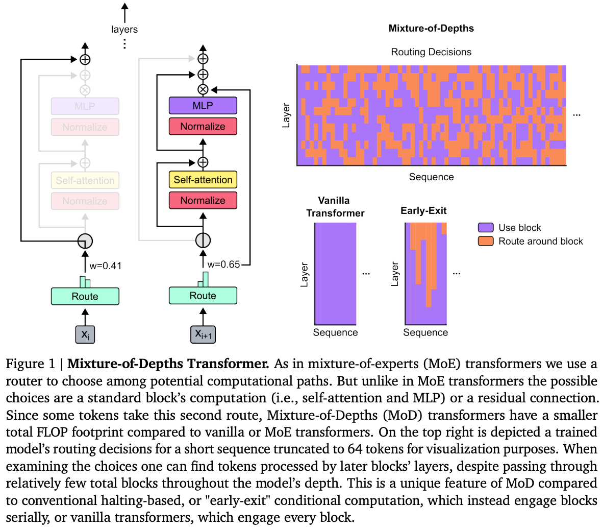
2024 Mixture-of-Depths: Dynamically allocating compute in transformer-based language models
Remember that MoEs work by subdividing the problem domain into smaller problems that are solved individually by different experts. In this paper, they claim that not all problems require the same amount of effort to train a model accurately. To that extent, they introduce Conditional computation, a technique that “tries to reduce total compute by expending it only when needed”. Here, “the network must learn how to dynamically allocate the available compute by making decisions per-token, in each layer, about where to spend compute from the available budget” - where this compute budget is a total number of FLOPs.
For every token, the model decides to either apply computation (as in the standard transformer), or skip computation and pass it through a residual connection (remaining unchanged and saving compute). Moreover, contrarily to MoEs, the routing is applied to both the feedforward network and the multi-head attention. In the multi-head routing, the router will not only decide on which tokens to update, but which tokens are made available to attend to. “We refer to this strategy as Mixture-of-Depths (MoD) to emphasize how individual tokens pass through different numbers of layers, or blocks, through the depth of the transformer”. In practice, during training, for every input, the router produces a scalar weight (importance) per token. The gating picks the top-\(k\) tokens per sentence per block to participate in the transformer block computation. \(k\) is a hyper-parameter that defined the max number of tokens passed to a block, thus the computation graph and tensor sizes remain static throughout the execution. Setting \(k\) allows one to trade off between performance and speed, for a given compute budget.
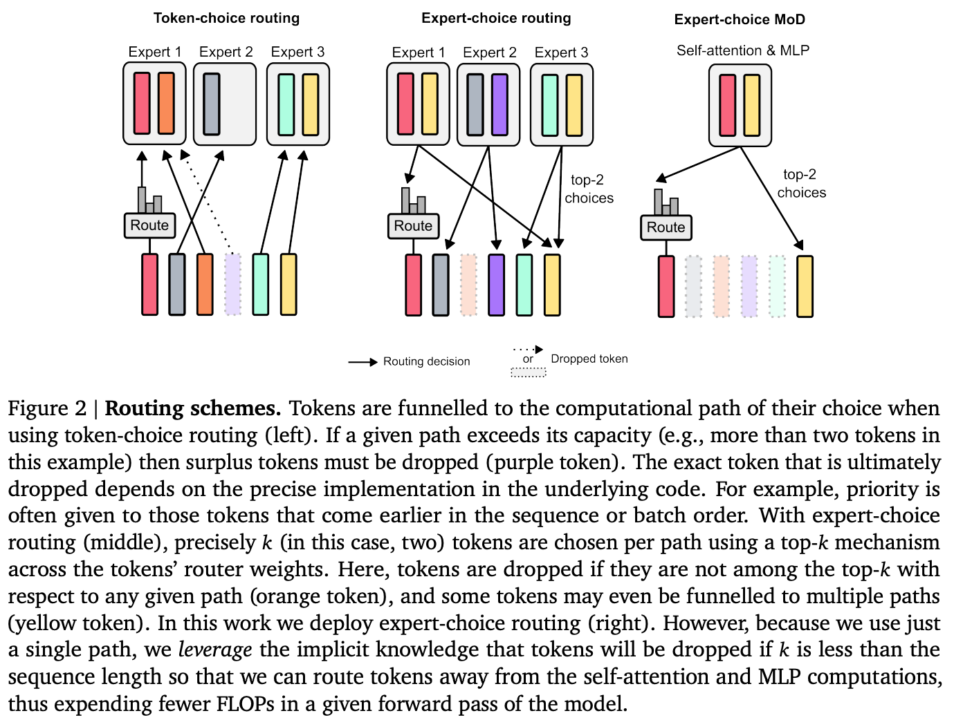
The big challenge is the routing scheme. The authors considered (1) token-choice where a router produces per-token probability distributions across computational paths (experts); and the orthogonal approach (2) expert-choice where instead of having tokens choose the expert they prefer, each expert instead picks the top-\(k\) tokens based on the tokens’ preferences. They ultimately adopted the expert-choice because it does not require load balancing, and “routers can try to ensure that the most critical tokens are among the top-\(k\) by setting their weight appropriately”.
At the time of writing of this post, this is still very recent work, so future will tell if MoDs become useful for the general use case.