Numerical Resolution of the Electrical Activity of Detailed Neuron Models
Neurons are a very complex structure of the human body that govern behaviour, pain, feelings, motion, and most factors that interfere with out human life. The human body has approximately \(8.6^{10}\) neurons, connected by \(1.5^{14}\) synapses. For the sake of comparison, larvae have 231 neurons, mice have approximately \(71\) Million neurons, and the african elephant has almost four times the human scale, with \(25.7^{10}\) neurons — see the wikipedia entry List of animals by number of neurons for a larger list neurons per mammal.
Due to very sophisticated anatomical structure and behaviour of neurons, we utilise numerical methods applied to approximation of neuron models in order to simulate the electrical activity on neural networks.

source: wikipedia
Hodgkin-Huxley Model and Cable Theory
The Hogkin-Huxley (HH) model(A. L. Hodgkin and A. F. Huxley, 1952) is built on several assumptions that disregard various features of the living cell and reduces the multidimensional complexity of the propagation and interaction of electrical signals in spatially extended nerve cells to a set of one dimensional constraints that fits the Cable Theory, a mathematical model to describe the changes in electric current and voltage along passive neurites.
A neuron’s membrane is formed by a phospholipid bilayer, a dielectric material, acting as a leaky capacitor. The cytoplasm inside the neurite (a part of a dendrite or axon) is considered to be an excellent ohmic conductor and the voltage within its membrane is assumed to be constant. The neurites are considered to be long and thin in such way that the voltage is assumed to vary much more along the long axis of the neural process than perpendicular to it. Therefore, diffusion of ions along the membrane surface and the dynamics of current perpendicular to the membrane are deemed irrelevant. The neuron morphology is simplified to a branched tree of interconnected neurites a length small enough to accept that the voltage across each neurite is constant. External to the neuron’s morphologies, certain mechanisms lead to electrical and chemical reactions that affect the potential of each individual capacitor. These mechanisms are typically gating channels, and allow the in/outflux of molecules (ions), that depolarize or hyperpolarise the membrane accordingly.
Another important mechanism are the synapses, which represent the interneural connections of the circuit. Synapses can drive the post-synaptic membrane potential upwards or downwards based on the excitatory or inhibitory properties of the pre-synaptic cell. Synapses are initiated when the potential of a membrane hits a particular Action Potential (AP) threshold, and is characterized by a stiff change of membrane potential. The lowest AP threshold on a neuron is typically at the beginning of the axon (the Axon Initial Segment), where synapses are first initiated. Other AP may happen throughout the axonal arborization as a current propagation mechanism. Synapses are driven by a fast influx of Sodium (\(Na^+\)) ions, and by the slow outflux of the Potassium (\(K^+\)) channels. The chlorine (\(Cl^-\)) conductance helps to bring the membrane potential back to the rest state following an activation. Several other mechanisms such as gap junctions (active electrical synapses), extracellular space mechanisms, or second messengers also exist. In the cable approximation model, the complexity of these mechanisms are reduced to the measurement of their ionic conductance. When the conductance of these molecules is constant, we call it a leak (passive) conductance. A compartment in ionic equilibrium, i.e. influx and outflux of neurons cause no variation of its potential, is said to be at its reversal potential.

The voltage trajectory during an Action Potential (spike)source: unknown
Mathematical Basis
The application of cable theory on the calculation of electrical signaling throughout neurons, resumes the activity of a neuron compartment to a second order partial differential equation that governs the change of axial current depending of time and distance, and reduces the relationship between current and voltage to a one-dimensional cable described by:
\[\frac{\partial V}{\partial T} + F(V) = \frac{\partial^2 V}{\partial X^2}. \label{equation338_neuronbook}\]Because the cable equation is linear and homogeneous, it obeys the superposition principle. The superposition principle states that, for all linear systems, the net response at given place and time caused by several stimuli, equals the sum of the responses of each stimulus individually. More general solutions suitable for branched neurons can be obtained by summing equations of this form, with an appropriate boundary condition. Neurons are represented as interconnected neurites with individual properties, later discretized in time and space to allow for a conversion into algebraic difference equations, which can be solved iteratively using numerical methods. For any given neurite, the principle of conversation of charge requires that the sum of currents from all sources must equal 0. The charge conservation principle states that electric charge can neither be created nor destroyed, and the amount of net quantity of electric charged given by sum of positive change and negative charge is always conserved. I.e.
\[\sum i_a - \int_A i_m dA = 0\]where \(i_a\) is the axial current [mA], flowing through the compartment’s region, and \(\int_A i_m dA\) is the transmembrane current density \(i_m\) [mA/cm\(^2\)] over the membrane area \(A\) [cm\(^2\)]. This concept is illustrated in the following picture:
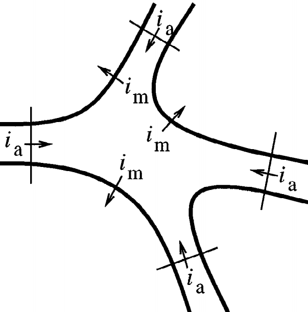
A common assumption is that a neuron is spatially divided into compartments small enough in such way that the spatially varying \(i_m\) is any compartment \(j\) is well approximated to the value on its center, therefore
\[\int_A i_{m_j} dA_j = i_{m_j} A_j = \sum_k i_{a_{kj}}\]Ohm’s law states that the current between two points of a conductor is directly proportional to the voltage across those two points, as described by the relationship \(I = V / R\). In order to resolve the axial current between a compartment \(j\) and its neighbors, we calculate the value based on Ohm’s where each axial current \(i_a\) is approximated by the voltage drop between the centers of the compartments and divided by the resistance of the path between them (the axial resistance), therefore:
\[i_{a_{kj}} = \frac{v_k - v_j}{r_{jk}}\]where \(r_{jk}\) represents the axial resistance i.e. the resistance of the path between the compartments \(k\) and \(j\). Finally, the total membrane current given by the sum of the capacitive and ionic components must equal the sum of axial currents \(i_{a_{kj}}\) that enter the compartment \(j\) from each adjacent neighbor \(k\), thus:
\[c_j \frac{dv_j}{dt}+i_{ion_j} (v_j, t) = i_{m_j}A_j \label{convervation_energy_eq}\]where \(c_j\) is the membrane capacitance of the compartment, \(c_j (dv_j / dt)\) the capacitive component, and \(i_{ion} (v_j, t)\) represents the ion channels conductances. Applying spatial discretazation to the equation of conservation of energy leads to a set of ordinary differential equations of the form:
\[c_j \frac{dv_j}{dt}+i_{ion_j} (v_j, t) = \sum_k \frac{v_k - v_j}{r_{jk}}. \label{equation345_neuronbook}\]We ommit from equation \ref{equation345_neuronbook} any injected source currents from the equation, which (if existent) is included on the right-hand side of the equation. If we consider the special case of an unbranched cable with constant parameter, the axial current is delimited by two points involving compartments \(j-1\) and \(j+1\) i.e.
\[c_j \frac{dv_j}{dt}+i_{ion_j} (v_j, t) = \frac{v_{j-1} - v_j}{r_{j-1,k}} + \frac{v_{j+1} - v_j}{r_{j+1,k}} \label{equation346_neuronbook}\]For a compartment with length \(\Delta x\) and diameter \(d\), the capacitance is given by \(C_m \pi d \Delta x\) and the axial resistance by \(R_a \frac{\Delta x}{\pi} (\frac{d}{2})^2\), where \(C_m\) is the membrane capacitance and \(R_a\) its cytoplasmic resistivity. Replacing those terms on equation \ref{equation346_neuronbook} leads to:
\[C_m \frac{dv_j}{dt}+i_{ion_j} (v_j, t) = \frac{d}{4Ra} \frac{v_{j+1} - 2 v_j + v_{j-1}}{ \Delta x^2} \label{equation347_neuronbook}\]If we assume the discretizaton variable to be small enough i.e. \(\Delta x \leftarrow 0\), using finite difference we wave the first derivative at the point in \(j\) given by \(\frac{v_j - v_{j-1}}{\Delta x}\) and \(\frac{v_{j+1} - v_j}{\Delta x}\), and the second-order correct approximation as
\[\frac{\partial^2v}{\partial x^2} = \left( \frac{v_{j+1} - v_j}{\Delta x} - \frac{v_j - v_{j-1}}{\Delta x} \right) \frac{1}{\Delta x} = \frac {v_{j+1} - 2v_j + v_{j-1}}{ \Delta x^2} \label{eq_2nd_order_finite_difference}\]we can replace this term in equation \ref{equation347_neuronbook}, where we get
\[C_m \frac{dv_j}{dt}+i_{ion_j} (v_j, t) = \frac{d}{4Ra} \frac{\partial^2v}{\partial x^2} \label{equation348_neuronbook}\]Following Ohm’s law we make the substitution \(i = v / R_m\), and multiply \(R_m\) on both sides, leading to the final formulation
\[R_m C_m \frac{dv_j}{dt} + v = \frac{d R_m}{4Ra} \frac{\partial^2v}{\partial x^2} \label{equation349_neuronbook}\]By substituting \(t = T \tau\) and \(x = X \lambda\) we scale equation \ref{equation349_neuronbook} to the time and space constants \(\tau = RC\) and \(\lambda = (1/2) \sqrt{d R_m / R_a}\), leading to a final formulation in the form of the Cable equation \ref{equation338_neuronbook}
Ionic Currents
All channels may be characterized by their resistance or by their conductance \(g = 1/R\), and by gating variables that add the open probability of a given channel, that generalizes external events that may block an ion channel. Hodgkin and Huxley formulated the ionic component components of a membrane as:
\[\sum_k I_k = g_{N_a} m^3 h (u - E_{Na}) + g_K n^4 (u - E_K) + g_L (u - E_L)\]where \(E\) represents the reversal potentials and \(m\), \(n\) and \(h\) the gating variables — see the original HH paper for details of individual ODEs and reported values. The leak generalizes any other voltage-independent conductance and is represented by \(L\).
Reversal Potential
The reversal potential for a particular ion flux in a compartment is given by the Nernst equation
\[E = \frac{RT}{zF} ln \frac{\text{[ion]}_{out}}{\text{[ion]}_{in}} \approx \frac{RT}{zF} 2.3026 \log _{10} \frac{\text{[ion]}_{out}}{\text{[ion]}_{in}}\]where \(ext{[ion]}_{out}\) and \(\text{[ion]}_{ion}\) denote the ionic concentration on the inside and outside of the cell, \(T\) is the temperature (Kelvin) (assumed to be \(307.15 K\) or \(34 ^{\circ}\mathrm{C}\)), \(z\) is the charge of the ion, and \(R\) and \(F\) are the Gas (\(8.3144621 J\) \(K^{-1}\) \(mol^{=1}\)) and Faraday constants (\(96485.33289(59)\) \(C\) \(mol-1\)) respectively. The typical reversal potential for the most common ions are approximately:
- \(E_{Cl^-}=-70 mV\) with \([Cl^-]_{in}=5 mM\) and \([Cl^-]_{out}=120 mM\);
- \(E_{K^+}=-90 mV\) with \([K^-]_{in}=150 mM\) and \([K^-]_{out}=4 mM\);
- \(E_{Na^+}=60 mV\) with \([Na^+]_{in}=12 mM\) and \([Na^+]_{out}=145 mM\); and
- \(E_{Ca^{2+}}=130 mV\) with \([Ca^{2+}]_{in}=0.1 mM\) and \([Ca^{2+}]_{out}=1 mM\).
The reversal potential of a typical HH compartment with \(Na^+\), \(K^+\) and \(Cl^-\) ionic pumps is given by the Goldman–Hodgkin–Katz flux equation as:
\[V = - \frac{RT}{F} ln \frac{P_{Na} [Na^+]_{out} + P_{K} [K^+]_{out} + P_{Cl} [Cl^-]_{in}} {P_{Na} [Na^+]_{in} + P_{K} [K^+]_{in} + P_{Cl} [Cl^-]_{out}} \approx -60 mV\]Boundary Conditions
The value of the normal derivative of the boundary function is a Neumann boundary condition assuming a neurite with a free ending point follows the form \(\frac{\partial v}{\partial x}=0\), i.e. no current flows on the terminal of a cable.
Branching Points
Branching points are modeled as idealized portions of the neurite that do not have membrane properties yet have axial current. Spatial discretization is equivalent to reducing the spatially distributed neuron to a set of connected compartments, and results on a set of ordinary differential equation that respect Kirchoff’s current law. Kirchoff’s current law, based on the principle of conservation of electric charge, states that the sum of currents entering any junction is equal to the sum of currents leaving that junction.
Numerical Resolution Methods in NEURON
Most equations that govern the brain mechanisms do not have an analytic solution. The NEURON simulator — henceforth referred to simple as NEURON — addresses such problems by allowing for a biologically realistic — not infinitely detailed — models of brain mechanisms, by utilizing several methods for accurate discretization of the neuronal activity into a discrete space.
The Hines Solver
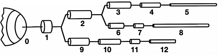
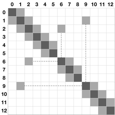
Due to the unique morphology of a cable model representation of a discretized neuron, NEURON implements an optimized linear solver for bifurcated trees, denominated as the Hines Algorithm (Efficient computation of branched nerve equations, Hines et al. Elsevier). Data is represented as a sparse tridiagonal matrix where the indices of the parent nodes (the ones immediately above on the tree structure) are provided by an extra vector \(p\). The membrane potential of each compartment is represented by the main diagonal. The contribution from a parent to its children compartments (and vice-versa) are represented by all cells on the same row (column) on the upper (lower) diagonal of the matrix. As each compartment can have only one parent, this enforces only one cell per row on the lower diagonal, and one cell per column on the upper diagonal. For completion, the followin pictures presents a neuron’s dendritic arborization spatially discretized based on the cable model (left) and its sparse matrix representation according to the Hines algorithm (right).
The main rationale behind the Hines algorithm is that if the we can number sequentially the compartments in such way that they all have an index greater than any of its children, then we can reduce the computational complexity of the solver from the \(O(n^3)\) found on a typical Gaussian elimination to \(O(n)\). Given a tridiagonal matrix with vectors \(d\) (main diagonal), \(b\) (lower diagonal) and \(a\) (upper diagonal), representing a single cable without branching, we can show that the Hines algorithm is an inverted Gaussian elimination adapted for branched structures:
- Starting with the forward triangulation process on each \(cell_i\) on row \(i\):
- \(cell_i \leftarrow cell_i \frac{b_i}{d_{i-1}} row_{i-1}\);
- Changing function variable from \(i\) to \(i+1\):
- \(cell_{i+1} \leftarrow cell_{i+1} \frac{b_{i+1}}{d_i} row_i\);
- Replacing forward by backward triangulation:
- \(cell_{i-1} \leftarrow cell_{i-1} \frac{a_{i-1}}{d_i} row_i\);
- Parent contributions for top node (\(a_0\) and \(b_0\)) do not exist:
- \(cell_{i-1} \leftarrow cell_{i-1} \frac{a_i}{d_i} cell_i\);
- Changing parents’ indices from single cable (\(i-1\)) to branched tree structure (\(p_i\)):
- \(cell_{p_i} \leftarrow cell_{p_i} \frac{a_i}{d_i} cell_i\);
which is the backwards triangulation applied. The substitution step in Hines is replaced by a forward substitution instead.
An important feature of the Hines algorithm is that it allows parallelization at the junction level, by starting the computation at the branches without children (terminal branches), the individual contributions from children branches can be computed in parallel, and included recursively at the parent compartment’s node.
Mechanisms and Events
In NEURON, extra-cellular activity, recording patches, voltage clamps, interneuron kinetics (such as synapses and gap junctions) or any other contribution that affects the membrane potential itself are introduced as mechanisms. A mechanisms with a specific execution time is called an event. Events in NEURON are managed by the event delivery delivery system (Efficient discrete event simulation of spiking neurons in NEURON, Carnevale et al., ResearchGate). Mechanisms are encoded in NMODL language Expanding NEURON’s Repertoire of Mechanisms with NMODL, Hines et al., where the main user-provided blocks are BREAKPOINT (the main computation block of the model where solves are integrated by a SOLVE statement), DERIVATIVE (if states are governed by differential equations, assigns values to the derivative), PROCEDURE and FUNCTION (function declaration and calls), PARAMETER and CONSTANT (for read-write and read-only variables, respectively) and NET_RECEIVE (a protocol to inform the variable time step scheduler that an event has occurred within the previous time step).
Fixed Time Stepping Interpolation
We showed previously that the principle of conversation of charge between two or more coupled compartments, including an external source of current injection \(I_{inj}\), can be stated by a set of equations of the form:
\[c_j \frac{dv_j}{dt}+i_{ion_j} (v_j, t) = \sum_k \frac{v_k - v_j}{r_{jk}} + I_{inj} \label{equation42_neuronbook}\]The resolution of the aforementioned based on numerical methods raises several concerns on stability, accuracy and efficiency, caused by the errors on the spatial discretization on the cable theory model and by the algorithms for resolution of the numerical solutions. This has been analyzed in The NEURON book, where the authors compare its numerical accuracy against the spatial discretization of the Fourier cosine terms \(cos ( \pi n x / L)\).
NEURON performs a spatial discretization of a compartment by placing \(m\) points on the center of equidistant intervals of size \(\Delta x = L /(m-1)\), thus each point is placed at \(x = (i+0.5) L/m\), for \(0 \geq i > m\). This is known (by numerical methods theory) to have higher accuracy when compared with the traditional method that places the \(m\) points at positions \(x = i \,\, L/(m-1)\) for \(0 \geq i \geq (m-1)\). In either case, \(m\) points are placed at a given compartment and \(m=1\) corresponds to spatial frequency of \(0\), i.e. uniform membrane potential along the entire cable. Also, the highest number of half waves that can be represented by the discretized system is \(n = m-1\), which is valid according to the Nyquist–Shannon sampling theorem. The Nyquist–Shannon sampling theorem establishes a condition for sufficient sampling rate of a discrete sequence of samples (digital information) to capture all the information from a continuous-time signal of finite bandwidth (analog information). In practice, it states that at least two samples must be captured per cycle in order to measure the frequency of a signal. The resolution of a spatially discretized compartment with respect to time follows a standard equation of a linear passive capacitor — a capacitor’s charge \(V\) at a given instante \(t\) is given by \(V = V_0 e^{-t / \tau}\) where the time constant \(\tau = RC\) and \(V_0\), \(R\) and \(C\) denote the initial charge, the capacitors resistance and capacitance, respectively — of the form:
\[\frac{dV_{nm}}{dt} = -k_{nm} V_{nm} \label{eq_310_neuronbook}\]where its analytic solution is
\[V_{nm} = V_{0_{nm}} e^{-k_{nm}t}\]and the rate constant \(k_{nm}\) is the inverse of the membrane time constant \(\tau _m = c/g\) for the point \(n\) of \(m\) points per compartment. The temporal discretization for a fixed time step approach follows the basic approximation principle for time stepping between two intervals:
\[\frac{d V}{d t} \approx \frac{V(t + \Delta t) - V(t)}{ \Delta t}\]Fixed time step interpolation is typically performed with either Euler or Crank-Nicholson methods. The explicit Forward Euler provides first-order accuracy and that the computational time step must never be more than twice the smallest constant on the system. As a reminder, a numerical solution to a differential equation is said to be of n\(^{th}\)-order if the error \(E\) is proportional to the \(n^{th}\) power of the step-size \(h\): \(E(h)=Ch^n\). The gap between the analytic and numerically solved solution is particularly high when the system’s voltage is changing rapidly, making it unstable. This has been described on detail in The NEURON book. For an extremely small time step \(\Delta t=0.0001 ms\) the system almost achieves equilibrium with the added cost of very high computation. Therefore Forward Euler is not applied in NEURON The Backward Euler method computes the solution of a set of nonlinear simultaneous equations at each step, therefore requiring a step size as large as possible to compensate for the extra work. For reasonable values of \(\Delta t\) it produces fast simulations that are very often generally correct, explained by the fact that tightly coupled compartments do not generate large error oscillations and approach the system’s equilibrium quickly. As its numerical error is proportional to \(\Delta t\) the Backward Euler does not deal with non-linearities. A function or map \(f(x)\) is said to be linear it satisfies the properties of superposition (\(f(x+y) = f(x) + f(y)\)) and homogeneity (\(f (\alpha x) = \alpha f (x)\)). The equation(s) of a non-linear system cannot be written as a linear combination of its unknown variables or functions.
The accuracy of the Backward Euler is improved by the Crank-Nicholson method, that provides a local error proportional to the square of the step size. As \(\Delta t\) becomes large, the solution oscillates with decreasing amplitude, making it numerically stable — see Hines et al. (1997) for a numerical resolution of passive compartments and action potential. Computation-wise, the Crank-Nicholson method is stable and more accurate than the Backward Euler, while requiring the same number of computation steps as Backward Euler. This can be shown by the following: if we take implicit (Backward) Euler to be defined as
\[y^{n+1}= y^n + \Delta t \,\, A y^{n+1} = (I - \Delta t \,\, A)^{-1} y^n\]and explicit (Forward) Euler as:
\[y^{n+1} = y^n + \Delta t \,\, A y^n = (I + \Delta t \,\, A) y^n\]then Crank-Nicholson can be described as:
\[y^{n+1} = y^n + \frac{1}{2}\Delta t \space{ } A y^{n+1} + \frac{1}{2}\Delta t \space{ } A y^{n} = \left( I - \frac{1}{2} \Delta t \,\, A \right)^{-1} \left(I + \frac{1}{2} \Delta t \,\, A \right) y^n\]which is 2 steps of implicit Euler, therefore requiring no extra computation for the added accuracy:
\[2 y^{n+1} - y^n = (2(I - \Delta t \,\, A)^{-1} - I) y^n = (I - \Delta t \space{ } A)^{-1} (I + \Delta t \space{ } A) y^n \label{eq_crank_nicholson_steps}\]Computational Implementation
NEURON’s workflow for the resolution based on interleaved time stepping is defined by a set of iterations that run sequentially for every computation and communication time step of duration \(\Delta t\) and \(\Delta t_{comm}\) respectively as:
- at instant \(t\):
- delivery of all (queued) spikes delivery for the subsequent iteration;
- channels run their mechanisms to deliver current;
- synaptic currents are delivered to the compartments;
- at instant \(t + \Delta t /2\):
- Linear algebra resolution via (Hines) solver;
- at instant \(t + \Delta t\):
- Update channels states;
- Update synapses states;
- Action Potential threshold detection;
- if \(t\) is a multiple of \(\Delta t_{comm}\):
- Perform collective call to send/recv spikes;
- Place all received spikes on spikes queue;
- Jump to next time step: \(t \leftarrow t + \Delta t\);
\(\Delta t\) is defined by the fastest mechanisms requiring no data exchange between compute nodes (normally the fastest \(Na^+\) channels). \(\Delta t_{comm}\) is fixed as the fastest mechanism requiring communication among compute nodes — typically the minimal synaptic delay across all synapses, or (when applicable) the update frequency for extra-cellular mechanisms or gap junctions.
NEURON’s implementation of fixed time step integrates the equation over the \(\Delta t\) step by calling all the BREAKPOINT blocks of the models at \(t + \Delta t /2\) twice with \(v\) and \(v+.001\) in order to compute the current and contribution of conductance from each mechanism, in order to form the matrix conductancevoltage=current. The matrix is then solved for \(v(t+ \Delta t)\). Lastly, in line with the staggered time stepping scheme, the *SOLVE statement of the models (within the BREAKPOINT block) is executed with \(t+ \Delta t\) and the new \(v\) in order to integrate those states, from the new \(t-\Delta t/2\) to new \(t+\Delta t/2\).
A strong argument supporting a fixed time step approach is the possibility of data vectorization. At every time step, several mechanisms run the same operations with different inputs, therefore allowing for a data layout in memory that takes advantage of hyperthreading or other vectorization modules on modern architectures.
Handling of non-linearity
Although nonlinear equations generally require an iterative resolution in order to maintain second order correcteness, the HH membrane properties allow the cable equation to be described linearly and solved without iterations, while keeping second-order error accuracy. NEURON’s variant of Crank-Nicholson with staggered time stepping applies the Strang splitting method to calculate the values of the compartment voltage and Hodgkin-Huxley gating states on interleaved time intervals. Therefore it converts a large non-linear system into two linear systems and the problem has now second-order accuracy, with a computation cost almost identical to the Backward Euler method. As a side note, a direct solution of voltage equation using a linearized membrane current \(I(V,t)=g(V-E)\) at a time step \(t \rightarrow t + \Delta t\) is possible if the conductance \(g\) and reversal potential \(E\) have second-order accuracy at time \(t+\Delta t/2\). as detailed in The NEURON book. Since the conduction of HH-type channels is given by a function of state variables \(n\) (\(K^+\)), \(m\) and \(h\) (\(Na^+\)), this second-order accuracy at \(t+\Delta t/2\) is achieved by performing a calculation with a time step offset of \(\Delta t/2\) from the current voltage time step. In brief, to calculate the second-order accurate integration between \(t-\Delta t/2\) and \(t+\Delta t/2\) we only need the second-order correct value of voltage-dependent rates at the instant \(t\).
\(\Delta t\) is defined by the fastest mechanisms requiring no data exchange between compute nodes (normally the fastest \(Na^+\) channels). \(\Delta t_{comm}\) is fixed as the fastest mechanism requiring communication among compute nodes — typically the minimal synaptic delay across all synapses, or (when applicable) the update frequency for extra-cellular mechanisms or gap junctions.
An important message here is that this resolution as a system is linear equations is only possible for simple models. Neuron models with non-linear state variable OPDEs and correlation between states require a fully-implicit resolution, and is possible with Backward Euler with Newton iterations. This is a common use case, and underlies the resolution of extra-cellular mechanisms, capacitors between nodes, and other mechanisms that connect neurons’ evolution over time. For such use cases, the regular Euler and Crank-Nicholson methods described previously have to be used, to the cost of a more computationally heavy simulation.