Faster Attention (Grouped, Latent, Sparse, Compressed and Linear)
The scaled dot-product attention of an attention head is computed as:
\[\text{Attention}(Q, K, V) = \text{softmax}\left( \frac{QK^T}{\sqrt{h}} \right) V\]where \(Q\), \(K\) and \(V\) are the queries, keys and values of the \(S\) tokens of a sequence, \(h\) is the head size, and the softmax turns each row of scores into weights that sum to one. Multi-head attention (MHA) runs \(H\) heads in parallel, each with its own projections of the input \(X\), and projects their concatenated outputs back to the embedding size \(E\):
\[\text{MHA}(X) = \left[ \text{head}_1, \dots, \text{head}_H \right] W^O, \quad \text{head}_i = \text{Attention}\left( X W^Q_i, X W^K_i, X W^V_i \right)\]where \(W^Q_i\), \(W^K_i\) and \(W^V_i\) are the \(E \times h\) projections of head \(i\), and \(W^O\) is the \(Hh \times E\) output projection.
As models and contexts grow, attention becomes the bottleneck, as its scores take \(O(S^2)\) time and memory. Prefill computes the full attention of the prompt, over all pairs of tokens. Decode computes only the attention of the new token, over the keys and values of the past tokens kept in the KV cache, which grows with the sequence length and with the number of layers and heads. So each decode step reads the whole cache, making KV cache the major culprit for decode being limited by memory bandwidth. Several efforts try to optimize this.
FlashAttention splits \(Q\), \(K\) and \(V\) into GPU tiles that fit in SRAM (few hundred KBs), and computes the scores, the softmax and the product with the values of each tile in a single kernel. As the softmax needs the maximum and the sum of a whole row, each query keeps a running maximum \(\mu\), sum \(\ell\) and unnormalized output \(o\), which are updated with each new tile of scores \(s_j\) and values \(v_j\) as:
\[\begin{align*} \mu' & = \max\left(\mu, \max_j s_j\right) \\ \ell' & = e^{\mu - \mu'} \, \ell + \sum_j e^{s_j - \mu'} \\ o' & = e^{\mu - \mu'} \, o + \sum_j e^{s_j - \mu'} \, v_j \end{align*}\]where \(j\) runs over the keys of the tile, \(e^{\mu - \mu'}\) rescales what was accumulated with the previous maximum, and the output is \(o / \ell\) after the last tile. Thus, the memory of attention drops from \(O(S^2)\) to \(O(S)\), and the backward pass recomputes the scores tile by tile, which is faster than reading them from HBM.
Other efforts like Flash-Decoding also split the KV cache along the sequence, so that decode, with a single query per sequence, uses the whole GPU. SageAttention quantizes the inputs of the two products of attention to 8 bits, and to 4 bits in its later versions. FlashInfer optimizes memory access and reduces redundancy through block-sparse formats: it uses Just-In-Time (JIT) compilation to adapt to various settings and employs a load-balanced scheduling algorithm to handle dynamic user requests efficiently.
Grouped-Query Attention (GQA)
MHA caches one key and one value per head. Multi-Query Attention (MQA) shares a single key and value head across all the query heads, which shrinks the KV cache \(H\) times, at some cost in quality. Grouped-Query Attention (GQA), used by most current models, is the middle ground: the \(H\) query heads are split into \(G\) groups that share one key and value head each, so the cache shrinks \(H / G\) times. GQA is MHA when \(G = H\), and MQA when \(G = 1\). The following picture illustrates it:
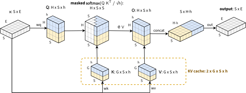
Grouped-query attention with H = 8 query heads in G = 4 groups: the two query heads of a group share one key head and one value head.
We can implement GQA by changing the original MHA and broadcasting the key and value tensor across the queries of each group:
class GQA(nn.Module):
    """ Grouped-Query Attention, causal: H query heads in G groups, each group sharing one key and one value head """

    def __init__(self, input_dim, head_dim, num_heads=8, num_groups=2):
        # [...] same as MHA
        self.num_groups = num_groups
        self.wq = nn.Linear(input_dim, head_dim * num_heads)   # one query per head
        self.wk = nn.Linear(input_dim, head_dim * num_groups)  # different than MHA: one key per group
        self.wv = nn.Linear(input_dim, head_dim * num_groups)  # different than MHA:  one value per group
        self.out = nn.Linear(head_dim*num_heads, input_dim)

    def forward(self, x):
        B, S, _ = x.shape
        H, G, h = self.num_heads, self.num_groups, self.head_dim
        R = H // G  # query heads per group

        # Instead of MHA's [B, H, S, h] dimension we add an extra dim for the head group
        q = self.wq(x).view(B, S, G, R, h).permute(0, 2, 3, 1, 4)  # [B, S, H*h] -> [B, G, R, S, h]
        k = self.wk(x).view(B, S, G, h).permute(0, 2, 1, 3).reshape(B, G, 1, S, h)  # [B, S, G*h] -> [B, G, 1, S, h]
        v = self.wv(x).view(B, S, G, h).permute(0, 2, 1, 3).reshape(B, G, 1, S, h)  # [B, S, G*h] -> [B, G, 1, S, h]

        causal_mask = torch.ones(S, S, dtype=torch.bool, device=x.device).tril()  # [S, S]
        scores = torch.einsum("bgrsh,bgrth->bgrst", q, k) * h**-0.5  # [B, G, R, S, h] @ [B, G, 1, S, h] -> [B, G, R, S, S]
        scores = scores.masked_fill(~causal_mask, float("-inf"))  # set to e^-inf=0 the masked values
        probs = scores.softmax(dim=-1)
        attn = torch.einsum("bgrst,bgrth->bgrsh", probs, v)  # [B, G, R, S, S] @ [B, G, 1, S, h] -> [B, G, R, S, h]
        attn = attn.permute(0, 3, 1, 2, 4).reshape(B, S, H * h)  # [B, G, R, S, h] -> [B, S, G, R, h] -> [B, S, H*h]
        return self.out(attn)
Multi-head Latent Attention (MLA)
In 2024, DeepSeek-V2 introduced Multi-head Latent Attention (MLA), which shrinks the KV cache further. MLA caches a small latent vector per token and recovers the keys and values of all heads from it with up-projections.
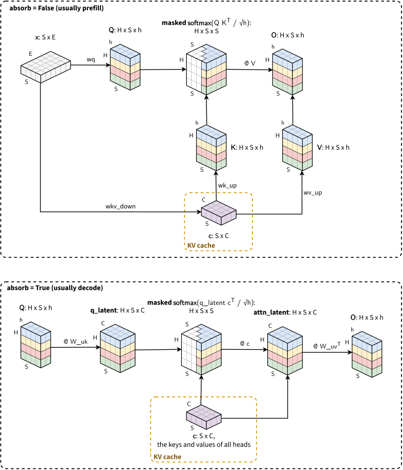
In prefill, it runs the naive mode (or MHA mode): it recovers the key \(k_{s,i} = c_s W^{UK}_i\) and the value \(v_{s,i} = c_s W^{UV}_i\) of each head \(i\) from the latent vector \(c_s\) of each token \(s\), and runs MHA. Prefill is compute-bound, and this mode needs fewer operations than the absorbed mode below: its scores and weighted sums use vectors of the head size \(h\), not the longer latent vectors. The following picture illustrates the naive mode:
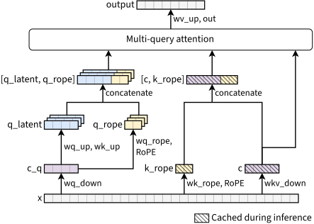
In decode, it runs the absorbed mode (or MQA mode), where attention runs directly over the cached latent vectors and reads far fewer values per token. The up-projections \(W^{UK}_i\) and \(W^{UV}_i\) of each head \(i\) are absorbed into its query and output, as:
\[q_i (k_{s,i})^T = \underbrace{q_i \left( W^{UK}_i \right)^T}_{\tilde{q}_i} (c_s)^T, \qquad \sum_s p_{s,i} v_{s,i} = \Big( \sum_s p_{s,i} c_s \Big) W^{UV}_i\]where \(q_i\) is the query of head \(i\) and \(p_{s,i}\) its softmax weight for token \(s\). Decode is memory-bound, and this mode reads only the cached latent vectors, shared by all heads. Rotary positional embeddings (RoPE) would prevent this absorption, as their rotation depends on the positions and sits between \(q_i\) and \(W^{UK}_i\). So MLA applies RoPE only to a small extra query per head and a key shared by all heads, cached with the latent vector. The following picture illustrates the absorbed mode:
The following code implements RoPE and MLA:
def rope(x, start=0, step=1, base=10000):
    # x: [..., S, D], D even: rotate each pair (2i, 2i+1) of the token at position m by angle m * base^(-2i/D)
    S, D = x.shape[-2:]
    theta = base ** (-torch.arange(0, D, 2, device=x.device) / D)  # [D/2] one frequency per pair
    m = start + step * torch.arange(S, device=x.device)            # [S] position m of every token: start, start + step, ...
    a = m[:, None] * theta                                         # [S, D/2] angle of every pair of every token
    x1, x2 = x[..., 0::2], x[..., 1::2]                            # [..., S, D/2] first and second element of each pair
    out = torch.empty_like(x)
    out[..., 0::2] = x1 * a.cos() - x2 * a.sin()
    out[..., 1::2] = x1 * a.sin() + x2 * a.cos()
    return out
class MLA(nn.Module):
    """ Multi-head Latent Attention, causal, with low-rank queries, a RoPE key shared by all heads and a KV cache """

    def __init__(self, input_dim, head_dim, num_heads=8, latent_dim=128, rope_dim=16):
        super().__init__()
        self.num_heads = num_heads
        self.wq_down = nn.Linear(input_dim, latent_dim)
        self.wkv_down = nn.Linear(input_dim, latent_dim)
        self.wq_up = nn.Linear(latent_dim, head_dim * num_heads)
        self.wk_up = nn.Linear(latent_dim, head_dim * num_heads)
        self.wv_up = nn.Linear(latent_dim, head_dim * num_heads)
        self.wq_rope = nn.Linear(latent_dim, rope_dim * num_heads)  # RoPE part of q, per head (rope_dim even)
        self.wk_rope = nn.Linear(input_dim, rope_dim)               # RoPE part of k, shared by all heads
        self.out = nn.Linear(head_dim * num_heads, input_dim)

    def attend_absorbed(self, q, q_rope, c, k_rope):
        """ One decode step with absorption: attention runs over the cached latent vectors, without building K and V """
        H, h, R = q.size(1), q.size(-1), q_rope.size(-1)  # q: [B, H, 1, h], q_rope: [B, H, 1, R]
        c, k_rope = c[:, None], k_rope[:, None]            # cache: [B, T, C] -> [B, 1, T, C], [B, T, R] -> [B, 1, T, R]
        W_uk = self.wk_up.weight.view(H, h, -1)            # [H*h, C] -> [H, h, C]
        W_uv = self.wv_up.weight.view(H, h, -1)            # [H*h, C] -> [H, h, C]
        q_latent = q @ W_uk                                # [B, H, 1, C]; the bias of the keys cancels in the softmax
        scores_latent = q_latent @ c.transpose(-1, -2)     # [B, H, 1, T]: the non-RoPE part, from the latent vectors
        scores_rope = q_rope @ k_rope.transpose(-1, -2)    # [B, H, 1, T]: the RoPE part, as in the naive mode
        scores = (scores_latent + scores_rope) / (h + R) ** 0.5  # [B, H, 1, T], scaled by 1/sqrt(h+R)
        attn_latent = F.softmax(scores, dim=-1) @ c        # [B, H, 1, T] @ [B, 1, T, C] -> [B, H, 1, C]
        attn = attn_latent @ W_uv.transpose(-1, -2) + self.wv_up.bias.view(H, 1, h)  # [B, H, 1, C] -> [B, H, 1, h]
        return self.out(attn.transpose(1, 2).reshape(q.size(0), 1, -1))  # [B, H, 1, h] -> [B, 1, H*h] -> [B, 1, E]

    def forward(self, x, kv_cache=None):
        B, S, _ = x.shape  # S: any length on prefill, 1 on decode
        H = self.num_heads
        P = 0 if kv_cache is None else kv_cache[0].size(1)  # number of cached tokens, before x

        head_out = lambda t: t.view(B, S, H, -1).transpose(1, 2)  # [B, S, H*D] -> [B, H, S, D]
        head_in = lambda t: t.transpose(1, 2).reshape(B, S, -1)   # [B, H, S, D] -> [B, S, H*D]

        c_q = self.wq_down(x)  # [B, S, E] -> [B, S, C]
        q = self.wq_up(c_q)  # [B, S, C] -> [B, S, H*h]

        ### Important: cached per layer: c [B, S, C] + RoPE key [B, S, R]; instead of K and V: 2 x [B, H, S, h]
        c = self.wkv_down(x)  # [B, S, E] -> [B, S, C]

        # RoPE part of q comes from c_q (per head), RoPE part of k from x (shared by all heads)
        # not applied to v: nothing would cancel its rotation, so the output would carry absolute positions
        q_rope = rope(head_out(self.wq_rope(c_q)), start=P)  # [B, H, S, R]
        k_rope = rope(self.wk_rope(x), start=P)              # [B, S, R]

        if kv_cache is not None:  # decode: append the new token to the KV cache, and attend in absorbed mode
            c = torch.cat([kv_cache[0], c], dim=1)            # [B, P+1, C]
            k_rope = torch.cat([kv_cache[1], k_rope], dim=1)  # [B, P+1, R]
            return self.attend_absorbed(head_out(q), q_rope, c, k_rope), (c, k_rope)

        k = self.wk_up(c)  # [B, S, C] -> [B, S, H*h]
        v = self.wv_up(c)

        causal_mask = torch.tril(torch.ones((S, S), dtype=torch.bool, device=x.device))

        # pull out head dimension: [B, S, H*D] -> [B, H, S, D]
        q, k, v = head_out(q), head_out(k), head_out(v)
        q = torch.cat([q, q_rope], dim=-1)                                 # [B, H, S, h+R]
        k = torch.cat([k, k_rope[:, None].expand(-1, H, -1, -1)], dim=-1)  # [B, H, S, h+R]

        # the final q, k and v: attention as in MHA
        out = F.scaled_dot_product_attention(q, k, v, attn_mask=causal_mask)  # [B, H, S, h], scaled by 1/sqrt(h+R)
        out = self.out(head_in(out))  # [B, S, H*h] -> [B, S, E]
        return out, (c, k_rope)

mla = MLA(input_dim=64, head_dim=16, num_heads=4, latent_dim=32, rope_dim=8)
x = torch.randn(2, 10, 64)                      # [B, S, E]
y, kv_cache = mla(x[:, :4])                     # prefill: the first 4 tokens at once, in naive mode
for t in range(4, x.size(1)):                   # decode: the next tokens, one per step, in absorbed mode
    y, kv_cache = mla(x[:, t:t + 1], kv_cache)  # the KV cache grows by one token per step
In DeepSeek-V2, MLA caches 57 times fewer values per token than MHA and 3.6 times fewer than GQA with 8 groups, and still performs better than MHA.
MLA with DeepSeek Sparse Attention (DSA)
MLA shrinks what each token stores, but each query still reads all the past tokens, which is costly for long contexts. DeepSeek-V3.2 is DeepSeek-V3.1 with DeepSeek Sparse Attention (DSA) added to its MLA by continued training. A lightning indexer scores the past tokens of each query with a small number of heads in FP8, and a top-k selector keeps only the \(k = 2048\) best-scored ones.
Attention then costs \(O(Sk)\) instead of \(O(S^2)\), and each decode step reads \(k\) cached tokens instead of \(S\), as a sparse kernel skips the other tokens. A mask gives the same output, but still computes all the scores and loads all the keys and values. The following picture illustrates both, with the tokens that the indexer selects:
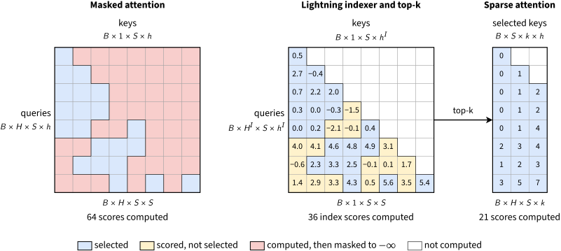
Masked attention (left), and the lightning indexer and the top-k selector, which pick the keys of sparse attention (right), with S = 8 tokens, k = 3 and indexer heads of size \(h^I\). The indexer scores the past tokens of each query, once for all heads, and selects the 3 best-scored ones. Sparse attention computes only their scores, an S × k matrix labeled with the positions of the selected keys. Masked and sparse attention keep the same 21 scores, but masked attention computes all 64.
The index score of a past token \(s\) for a query token \(t\) is computed as:
\[I_{t,s} = \sum_{j=1}^{H^I} w^I_{t,j} \cdot \text{ReLU}\left( q^I_{t,j} \cdot k^I_s \right)\]where \(H^I\) is the number of indexer heads, \(q^I_{t,j}\) and \(w^I_{t,j}\) are the query and the weight of head \(j\), and \(k^I_s\) is the indexer key of token \(s\), shared by all heads. The following picture illustrates MLA with DSA:
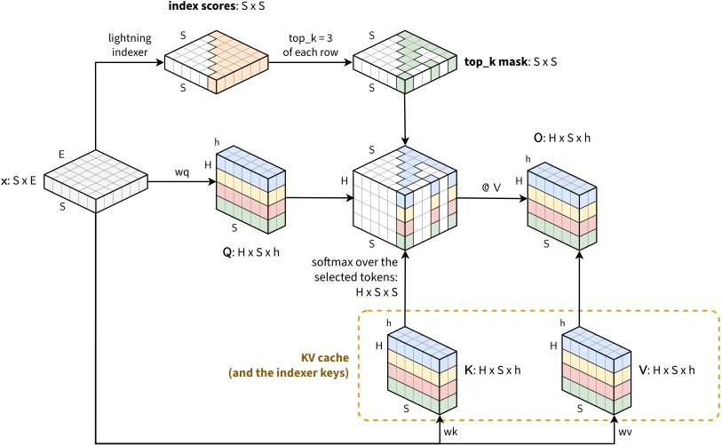
DeepSeek-V3.2: MLA with DSA. The lightning indexer and the top-k selector (red) pick the past tokens that the multi-head attention attends to, with the names of the code below.
The indexer still scores all pairs of tokens, but with much less computation than dense MLA. It is first trained alone to imitate the attention of its layer, with a KL-divergence loss, and then the whole model is trained with sparse attention.
DeepSeek-V3.2 runs DSA in the absorbed mode of MLA, also in prefill (Section 2.1 in the paper):
At the kernel level, each key-value entry must be shared across multiple queries for computational efficiency. Therefore, we implement DSA based on the MQA mode of MLA, where each latent vector (the key-value entry of MLA) will be shared across all query heads of the query token.
As each query token selects its own \(k\) tokens, only its heads can share what it loads: the absorbed mode loads one latent vector per selected token for all heads, while the naive mode loads a key and a value for each head. Only the prefill of short prompts runs the naive mode, with a mask, as it is faster for short contexts (Section 2.3 in the paper).
The following code implements DSA as a subclass of MLA that adds the lightning indexer and the top-k selector. Attention then reads only the latent vectors and RoPE keys of the selected tokens, in absorbed mode, as in attend_absorbed:
class DSA(MLA):
    """ MLA with DeepSeek Sparse Attention: a lightning indexer picks the top_k past tokens of each query token """

    def __init__(self, input_dim, head_dim, num_heads=8, latent_dim=128, rope_dim=16, index_heads=4, index_dim=32,
                 top_k=2048):
        super().__init__(input_dim, head_dim, num_heads, latent_dim, rope_dim)  # the weights of MLA
        self.top_k = top_k
        self.index_wq = nn.Linear(latent_dim, index_heads * index_dim)  # query of each indexer head, from c_q
        self.index_wk = nn.Linear(input_dim, index_dim)  # key of each token, shared by all indexer heads
        self.k_norm = nn.LayerNorm(index_dim)
        self.index_w = nn.Linear(input_dim, index_heads)  # weight of each indexer head

    def lightning_indexer(self, x, q_index, k_index, mask):
        """ Lightning indexer and top-k selector: the top_k best-scored keys in mask of each query, -1 for none """
        # lightning indexer: I[t, s] = sum_j w[t, j] * relu(q_index[t, j] . k_index[s])
        votes = F.relu(q_index @ k_index[:, None].transpose(-1, -2))  # [B, HI, S, N], relevance vote of each head
        w_index = self.index_w(x).transpose(1, 2)[..., None]  # [B, S, HI] -> [B, HI, S, 1]: weight w[t, j] of each head
        I = (w_index * votes).sum(1)  # [B, HI, S, 1] * [B, HI, S, N] -> sum over heads -> [B, S, N]

        # top-k selector: each query t keeps its k best-scored keys in mask, and -1 where it has fewer than k
        score, top = I.masked_fill(~mask, float('-inf')).topk(min(self.top_k, I.size(-1)), dim=-1)  # [B, S, k]
        return top.where(score > float('-inf'), -1)  # [B, S, k], with k = min(top_k, N)
Native Sparse Attention. NSA, published by DeepSeek before DSA, is trained with sparse attention from the start (natively). It selects blocks of 64 tokens rather than single tokens, as GPUs load contiguous blocks faster, and mixes three branches with learned gates: compressed blocks, the selected blocks that score highest in the compressed branch, and a sliding window over the last tokens.
Compressed Sparse Attention (CSA) and Heavily Compressed Attention (HCA)
MLA and DSA addressed different parts of the attention problem: MLA compresses the KV cache, so that the model does not store the full keys and values of every head and token; DSA reduces the number of tokens that the model attends to, with a learned selection.
As a follow-up, DeepSeek-V4 presents compressed attention, which focuses on extending the context to one million tokens, where the KV cache of MLA and the indexer of DSA, which scores every past token, become the bottleneck. So it compresses the KV cache along the sequence, with two types of attention that alternate after the first two layers (counted from zero):
- Compressed Sparse Attention (CSA), on the even layers, compresses every \(m = 4\) tokens into one KV entry, a weighted sum of their KV entries, and a lightning indexer picks the top-k entries of each query, as in DSA.
- Heavily Compressed Attention (HCA), on the odd layers, compresses every \(m = 128\) tokens into one entry in the same way, and attends to all of them.
Both also attend to the uncompressed KV entries of the last \(n_\text{win} = 128\) tokens, in a sliding window, to increase the attention detail on recent tokens. The attention runs one softmax over both sets of entries. In HCA, a token-level compressor computes the entry of block \(i\), a weighted sum of the KV entries of its \(m\) tokens, as:
\[C^\text{Comp}_i = \sum_{j=mi}^{m(i+1)-1} S_j \odot C_j, \qquad S_{mi:m(i+1)-1} = \text{softmax}\left( Z_{mi:m(i+1)-1} + B \right)\]where the rows of \(C = XW^{KV}\) and \(Z = XW^Z\), both \(n \times c\), are the KV entries and the compression weights of the \(n\) tokens, \(B\) is a learned \(m \times c\) positional bias, and \(\odot\) is the element-wise product. The softmax runs over the \(m\) tokens of the block, separately for each of the \(c\) channels. Each entry is both the key and the value of a single KV head, as in MQA.
In CSA, each entry also covers the previous block, with a second series of KV entries, weights and bias (Eq. 11 and 12 in the paper):
\[C^\text{Comp}_i = \sum_{j=mi}^{m(i+1)-1} S^a_j \odot C^a_j + \sum_{j=m(i-1)}^{mi-1} S^b_j \odot C^b_j\]where the series \(a\) covers block \(i\), the series \(b\) covers block \(i-1\), and one softmax runs over the \(2m\) weights of each channel. Thus, the entries overlap, but there is still one entry every \(m\) tokens. The indexer scores the entries as in DSA, with keys \(K^{I\text{Comp}}_s\) compressed in the same way, and keeps the top \(k\) (512 in DeepSeek-V4-Flash and 1,024 in DeepSeek-V4-Pro). As in MLA, the queries \(q\) of the attention and \(q^I\) of the indexer come from a low-rank latent vector \(c^Q\). The following picture illustrates CSA and HCA:
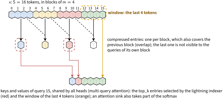
DeepSeek-V4: CSA and HCA for the query token t, with the symbols of the formulas above. The lightning indexer and the top-k selector (red), which pick the compressed entries that the attention reads with the window, are only in CSA. CSA has m = 4, and HCA has m = 128.
The following picture shows the attention scores (\(QK^T\)) of CSA and HCA, with the compression of their keys, and of the sliding window:
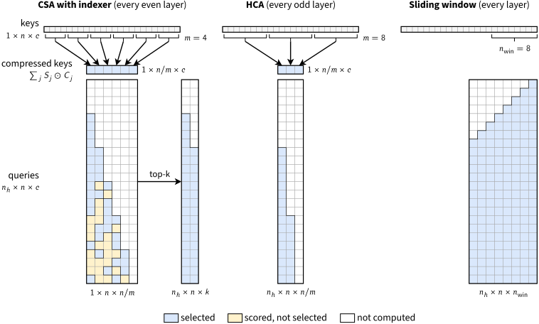
Attention scores of n = 24 tokens in CSA (m = 4, k = 2), HCA (m = 8) and the sliding window (n_win = 8), with HCA’s m and n_win scaled down from 128 to fit. Each compressed key is a weighted sum of the m keys of a block, and of the previous block in CSA, and a query sees only the blocks before its own. In CSA, the indexer scores these blocks once for all heads, with its own keys compressed in the same way, and attention computes only the scores of the 2 best-scored ones, an n × k matrix. The window computes the scores of the last n_win keys of each query, an n × n_win matrix.
The following code implements CSA, HCA and the auxilian methods to perform compresssion, sliding sliding and sparse attention:
R = 64  # RoPE channels: the last R of each query and KV entry, as in DeepSeek-V4
partial_rope = lambda x, step=1: torch.cat([x[..., :-R], rope(x[..., -R:], step=step)], dim=-1)

def compress(x, wkv, wz, bias, m, overlap=False):
    """ Token-level compressor: one KV entry per block of m tokens of x, over 2m tokens with overlap (CSA) """
    N = x.size(1) // m
    x = x[:, :N * m]  # the tokens of an incomplete last block wait until it is complete
    C = wkv(x).unflatten(1, (N, m))  # [B, N, m, h]: the KV entries of the tokens, in blocks of m
    Z = wz(x).unflatten(1, (N, m)) + bias  # [B, N, m, h]: their compression weights, plus the positional bias [m, h]
    if overlap:  # CSA: 2h channels instead of h, and the second h of block i - 1 also go into entry i
        (C, C2), (Z, Z2) = C.chunk(2, dim=-1), Z.chunk(2, dim=-1)
        C = torch.cat([C, F.pad(C2, (0, 0, 0, 0, 1, 0))[:, :N]], dim=2)  # [B, N, 2m, h]: blocks i and i - 1
        Z = torch.cat([Z, F.pad(Z2, (0, 0, 0, 0, 1, 0), value=float('-inf'))[:, :N]], dim=2)  # none before block 0
    entries = (Z.softmax(dim=2) * C).sum(dim=2)  # softmax over the tokens of each block, per channel: [B, N, h]
    return partial_rope(entries, step=m)  # entry i at position m * i, of the first token of block i

def sliding_window(kv, n_win=128):
    """ The uncompressed KV entries kv [B, S, h] that each query token t reads: the last n_win tokens, t included """
    t = torch.arange(kv.size(1), device=kv.device)[:, None]  # [S, 1]
    s = t - n_win + 1 + torch.arange(n_win, device=kv.device)  # [S, n_win]: tokens t - n_win + 1 to t
    return s.clamp(min=-1).expand(kv.size(0), -1, -1)  # [B, S, n_win]: their positions, -1 before the first token

def sparse_attention(q, kv, idx):
    """ MQA in which each query token reads only the entries of kv [B, L, h] that idx [B, S, K] lists, -1 for none """
    keys = kv[torch.arange(kv.size(0), device=kv.device)[:, None, None], idx.clamp(min=0)]  # [B, S, K, h]: a gather
    mask = (idx >= 0)[:, :, None]  # [B, S, 1, K]: the same for all the heads of a query token
    y = F.scaled_dot_product_attention(q.transpose(1, 2), keys, keys, attn_mask=mask)  # [B, S, H, h], from S x K scores
    return y.transpose(1, 2)  # [B, H, S, h]
and
class CSA_HCA(nn.Module):
    """ Compressed Sparse Attention (CSA), or Heavily Compressed Attention (HCA) with csa=False """
    lightning_indexer = DSA.lightning_indexer  # the indexer and top-k selector of DSA, over the compressed entries

    def __init__(self, input_dim, head_dim, latent_dim, index_heads, index_dim, m=4, top_k=512, csa=True):
        super().__init__()
        self.m, self.top_k, self.index_heads, self.csa = m, top_k, index_heads, csa
        dim = 2 * head_dim if csa else head_dim  # CSA: 2h channels, for the blocks i and i - 1
        self.wkv = nn.Linear(input_dim, dim)  # W^KV of the compressor
        self.wz = nn.Linear(input_dim, dim)  # W^Z
        self.bias = nn.Parameter(torch.zeros(m, dim))  # B
        if csa:  # the lightning indexer, with its keys compressed in the same way
            self.index_wkv = nn.Linear(input_dim, 2 * index_dim)
            self.index_wz = nn.Linear(input_dim, 2 * index_dim)
            self.index_bias = nn.Parameter(torch.zeros(m, 2 * index_dim))
            self.index_wq = nn.Linear(latent_dim, index_heads * index_dim)  # query of each indexer head, from c_q
            self.index_w = nn.Linear(input_dim, index_heads)  # weight of each indexer head

    def forward(self, x, c_q):
        entries = compress(x, self.wkv, self.wz, self.bias, self.m, overlap=self.csa)  # [B, N, h]
        (B, S, _), N = x.shape, entries.size(1)
        visible = torch.arange(N, device=x.device) < torch.arange(S, device=x.device)[:, None] // self.m  # [S, N]
        if self.csa:  # CSA: each query token reads the top_k entries of the lightning indexer
            k_index = compress(x, self.index_wkv, self.index_wz, self.index_bias, self.m, overlap=True)  # [B, N, DI]
            q_index = self.index_wq(c_q).view(B, S, self.index_heads, -1).transpose(1, 2)  # [B, HI, S, DI], as in DSA
            idx = self.lightning_indexer(x, partial_rope(q_index), k_index, visible)  # [B, S, k]
        else:  # HCA: each query token reads all the entries before its block
            idx = torch.arange(N, device=x.device).where(visible, -1).expand(B, S, N)  # [B, S, N]
        return entries, idx  # -1 for none
With a context of one million tokens, DeepSeek-V4-Pro needs 27% of the per-token inference FLOPs and 10% of the KV cache of DeepSeek-V3.2.
Linear attention
Softmax attention, formulated as \(\text{softmax}(QK^T) V\), keeps a KV cache that grows with the context, and its prefill computes the scores of all pairs of tokens. Softmax attention requires the softmax to be applied to each element of the \(S \times S\) matrix \(QK^T\). Linear attention showed that by replacing the softmax function with a kernel function \(\phi(\cdot)\), we can use the associative property of matrix multiplication to change the order of operations onto \(\text{Linear Attention} = Q (K^T V)\).
Here’s how. Without the causal mask, the output \(A_i\) of the query token \(i\), i.e. row \(i\) of the output \(A\), is derived as:
\[\begin{aligned} A &= \text{softmax}(QK^T) \, V && \text{softmax attention (Eq. 2)} \\ A_i &= \sum_{j=1}^{S} \text{softmax}(QK^T)_{ij} \, V_j && \text{row } i \text{ of } A \\ &= \sum_{j=1}^{S} \frac{e^{Q_i (K_j)^T}}{\sum_{k=1}^{S} e^{Q_i (K_k)^T}} \, V_j && \text{softmax of row } i \text{, with } (QK^T)_{ij} = Q_i (K_j)^T \\ &= \frac{\sum_{j=1}^{S} e^{Q_i (K_j)^T} \, V_j}{\sum_{j=1}^{S} e^{Q_i (K_j)^T}} && \text{the denominator does not depend on } j \end{aligned}\]where \(Q_i\), \(K_j\) and \(V_j\) are the rows \(i\) and \(j\) of \(Q\), \(K\) and \(V\), i.e. the query, key and value of the tokens \(i\) and \(j\). The dot product \(Q_i (K_j)^T\) is a similarity between the query and the key, and the last line is an average of the values weighted by its exponential. Any non-negative similarity function \(\text{sim}(Q_i, K_j)\) can replace this exponential, as (Eq. 3):
\[A_i = \frac{\sum_{j=1}^{S} \text{sim}(Q_i, K_j) \, V_j}{\sum_{j=1}^{S} \text{sim}(Q_i, K_j)}\]which is equivalent to Eq. 2 for \({\text{sim}(Q_i, K_j) = e^{Q_i (K_j)^T}}\). Linear attention uses instead a kernel, the dot product of two feature maps, \({\text{sim}(Q_i, K_j) = \phi(Q_i) \, \phi(K_j)^T}\), where \({\phi(x) = \text{elu}(x) + 1}\) applies to each element of a vector and keeps the weights positive. Other feature maps are ReLU (cosFormer) and positive random features that approximate the exponential (Performer). The output is then computed as (Eq. 4):
\[A_i = \frac{\sum_{j=1}^{S} \phi(Q_i) \, \phi(K_j)^T \, V_j}{\sum_{j=1}^{S} \phi(Q_i) \, \phi(K_j)^T}\]As matrix products are associative, \(\phi(Q_i)\) moves out of both sums, as (Eq. 5):
\[A_i = \frac{\phi(Q_i) \sum_{j=1}^{S} \phi(K_j)^T \, V_j}{\phi(Q_i) \sum_{j=1}^{S} \phi(K_j)^T}\]For all queries at once, the numerator is written in matrix form as (Eq. 6):
\[\left( \phi(Q) \, \phi(K)^T \right) V = \phi(Q) \left( \phi(K)^T V \right)\]where the left side computes the \(S \times S\) weights, as softmax attention does, and the right side only the \({h \times h}\) matrix \({\phi(K)^T V = \sum_j \phi(K_j)^T V_j}\), computed once and reused for every query in Eq. 5, as is the sum \(\sum_j \phi(K_j)^T\) of the denominator. Thus, attention takes \(O(S h^2)\) time instead of \(O(S^2 h)\), i.e. linear in \(S\).
Causal Mask
With the causal mask, the query token \(i\) attends only to the tokens up to \(i\), so the sums of Eq. 3 run up to \(i\) instead of \(S\) (Eq. 8):
\[A_i = \frac{\sum_{j=1}^{i} \text{sim}(Q_i, K_j) \, V_j}{\sum_{j=1}^{i} \text{sim}(Q_i, K_j)}\]As in Eqs. 4 and 5, the kernel replaces \(\text{sim}\), and \(\phi(Q_i)\) moves out of both sums (Eq. 9):
\[A_i = \frac{\phi(Q_i) \sum_{j=1}^{i} \phi(K_j)^T \, V_j}{\phi(Q_i) \sum_{j=1}^{i} \phi(K_j)^T}\]These prefix sums differ for each query, unlike the matrix \(\phi(K)^T V\) that all queries share without the mask, and are defined as (Eqs. 10 and 11, named \(S_i\) and \(Z_i\) in the paper):
\[\begin{aligned} M_i &= \sum_{j=1}^{i} \phi(K_j)^T \, V_j = M_{i-1} + \phi(K_i)^T \, V_i \\ z_i &= \sum_{j=1}^{i} \phi(K_j) = z_{i-1} + \phi(K_i) \end{aligned}\]where the state \(M_i\) is an \(h \times h\) matrix that sums the outer products of the keys and the values of the tokens up to \(i\), and \(z_i\) sums their keys, to normalize the weights. Each state is computed from the previous one in \(O(h^2)\) time, independent of \(i\), so the causal mask keeps the time linear in \(S\). Eq. 9 then simplifies to (Eq. 12):
\[A_i = \frac{\phi(Q_i) \, M_i}{\phi(Q_i) \, (z_i)^T}\]Thus, as Section 3.4 of the paper shows, a transformer layer with causal linear attention is a recurrent neural network (RNN): each token updates an internal state, \(M_i\) and \(z_i\), from which the layer computes its output. Linear attention combines the best of both, which makes the generation of long sequences thousands of times faster than with softmax attention (Section 3.3.2). In training and prefill, the states of all tokens are prefix sums, computed in parallel, as a transformer does. In decode, each layer keeps this state instead of a KV cache, which grows with the context, so its memory and its time per token stay constant, as in an RNN. The following picture illustrates it:
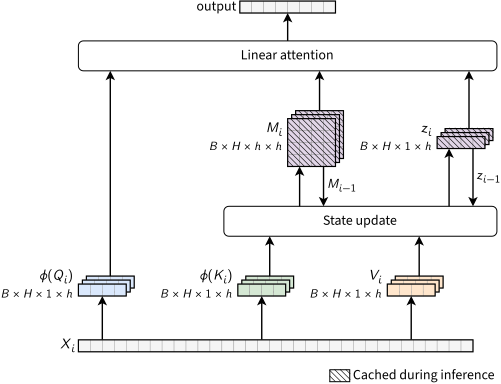
Linear attention for the token i in decode, with the symbols of the formulas above.
The following code implements linear attention with the causal mask. In prefill, the causal mask becomes a cumulative sum over the tokens, which gives the states \(M_i\) and \(z_i\) of all tokens at once. In decode, each new token updates the state of the past tokens:
class LinearAttention(GQA):
    """ Linear attention, causal, with the feature map elu(x) + 1 and a state of fixed size for decode """

    def __init__(self, input_dim, head_dim, num_heads=8):
        super().__init__(input_dim=input_dim, head_dim=head_dim, num_heads=num_heads, num_groups=num_heads)

    def forward(self, x, state=None):
        B, S, _ = x.shape  # S: any length on prefill, 1 on decode
        H = self.num_heads
        head_out = lambda t: t.view(B, S, H, -1).transpose(1, 2)  # [B, S, H*h] -> [B, H, S, h]
        head_in = lambda t: t.transpose(1, 2).reshape(B, S, -1)   # [B, H, S, h] -> [B, S, H*h]
        q, k, v = head_out(self.wq(x)), head_out(self.wk(x)), head_out(self.wv(x))  # same as MHA, GQA

        phi_q = F.elu(q) + 1  # [B, H, S, h]: feature map of each query
        phi_k = F.elu(k) + 1  # [B, H, S, h]: feature map of each key

        # causal mask: a cumulative sum over the tokens gives the states M_i and z_i of every token i
        M = (phi_k[..., :, None] * v[..., None, :]).cumsum(dim=2)  # [B, H, S, h, h]: sum of outer products up to i
        z = phi_k.cumsum(dim=2)                                     # [B, H, S, h]: sum of the keys up to i
        if state is not None:  # decode: add the state of the past tokens
            M, z = M + state[0][:, :, None], z + state[1][:, :, None]

        num = (phi_q[..., None, :] @ M).squeeze(-2)  # [B, H, S, 1, h] @ [B, H, S, h, h] -> [B, H, S, h]
        den = (phi_q * z).sum(dim=-1, keepdim=True)  # [B, H, S, 1]
        out = self.out(head_in(num / den))           # [B, H, S, h] -> [B, S, H*h] -> [B, S, E]
        return out, (M[:, :, -1], z[:, :, -1])       # state after the last token: [B, H, h, h] and [B, H, h]
For simplicity, this prefill stores the state of every token, i.e. \(S\) matrices of size \(h \times h\) per head. Optimized kernels split the sequence into chunks and keep only the state at the end of each chunk.
However, a state of fixed size holds at most \(h\) orthogonal keys, so it recalls a long context less precisely than a KV cache. Recent models add to the state update a data-dependent decay (Mamba-2), which forgets old tokens, the delta rule (DeltaNet), which replaces the value stored for a key, or both (Gated DeltaNet, Kimi Delta Attention). Hybrid models also interleave a few softmax attention layers with the linear ones, as their KV cache recalls exact tokens.
The decay relates linear attention to state space models (SSMs) such as Mamba, whose state of fixed size also decays at each token by a factor computed from the token. Mamba-2 shows that an SSM with a scalar decay \(\gamma_i\) per token is linear attention with the state update \(M_i = \gamma_i M_{i-1} + \phi(K_i)^T V_i\), without the normalization.