Efficient inference: prefill vs decode, roofline, KV cache, continuous/ragged batching, disaggregation
The goal of inference optimiztion to generate text as fast and as cheaply as possible, with a small memory footprint, and with little or no loss of quality. This matters for real-time and embedded systems, and for any service where the cost per generated token adds up. We will focus on the performance and implement the discussed methods on the same GPTlite model as before.
Prefill and decode phases
A GPT-like model generates text autoregressively: it reads the prompt, predicts the next token, appends it to the input, and repeats. Inference therefore has two phases that behave very differently:
- Prefill processes all the prompt tokens in a single forward pass. The tokens are processed in parallel, so the GPU performs large matrix-matrix multiplications and is compute-bound. Prefill ends with the first generated token, so its duration is the time to first token (TTFT).
- Decode generates the remaining tokens, one forward pass per token. Because of the Key-Value (KV) cache method we will detail later, each pass processes a single new token per sequence, so the GPU performs matrix-vector multiplications: it reads every weight of the model from memory to do very little arithmetic with it. Decode is memory-bandwidth-bound, and the duration of each step is the time per output token (TPOT), also called inter-token latency (ITL).
- Thus, the total runtime is given by the time to last token (TTLT) as \(\text{TTLT} = \text{TTFT} + \text{TPOT} \times ( n - 1)\), where \(n\) is the number of output tokens.
This observation explains most of this post. Almost every decode optimization does one of three things:
- it reads fewer bytes per token (quantization, smaller KV caches, smaller models), or
- it does more useful work per byte read (batching, speculative decoding), or
- it removes overheads around the math (kernel fusion, CUDA graphs, better scheduling).
Where does the compute goes, MLP versus attention
For a model of width \(d\) (the embedding size) and a context of \(n\) tokens, each layer spends, for every token:
- a term in the order of \(O(d^2)\) for the projections and the MLP;
- a term in the order of \(O(nd)\) for the attention scores \(QK^T\) and the weighted sum of the values.
The first term does not depend on the context length; the second grows with every token in the context. So attention becomes the dominant cost as the sequence length \(n\) increases. Memory follows the same pattern as computation. The model weights are read once per decode step and shared by all the sequences of the batch, while each sequence keeps its own cache of attention keys and values (KV cache) that grows with every token. For long contexts and large batches, reading the KV cache dominates the memory traffic and runtime of each decode step.
Roofline model
The roofline model, turns this calculation into a picture. It describes the computational performance as the number of FLOPs it performs per byte that moves between memory and the processor. A Roofline chart is plotted on a Log-Log scale, where:
- X-Axis (Arithmetic Intensity): How many math operations you perform per byte of data moved (FLOPs/byte).
- Y-Axis (Attainable Performance): How fast your code actually runs (GFLOPs/s).
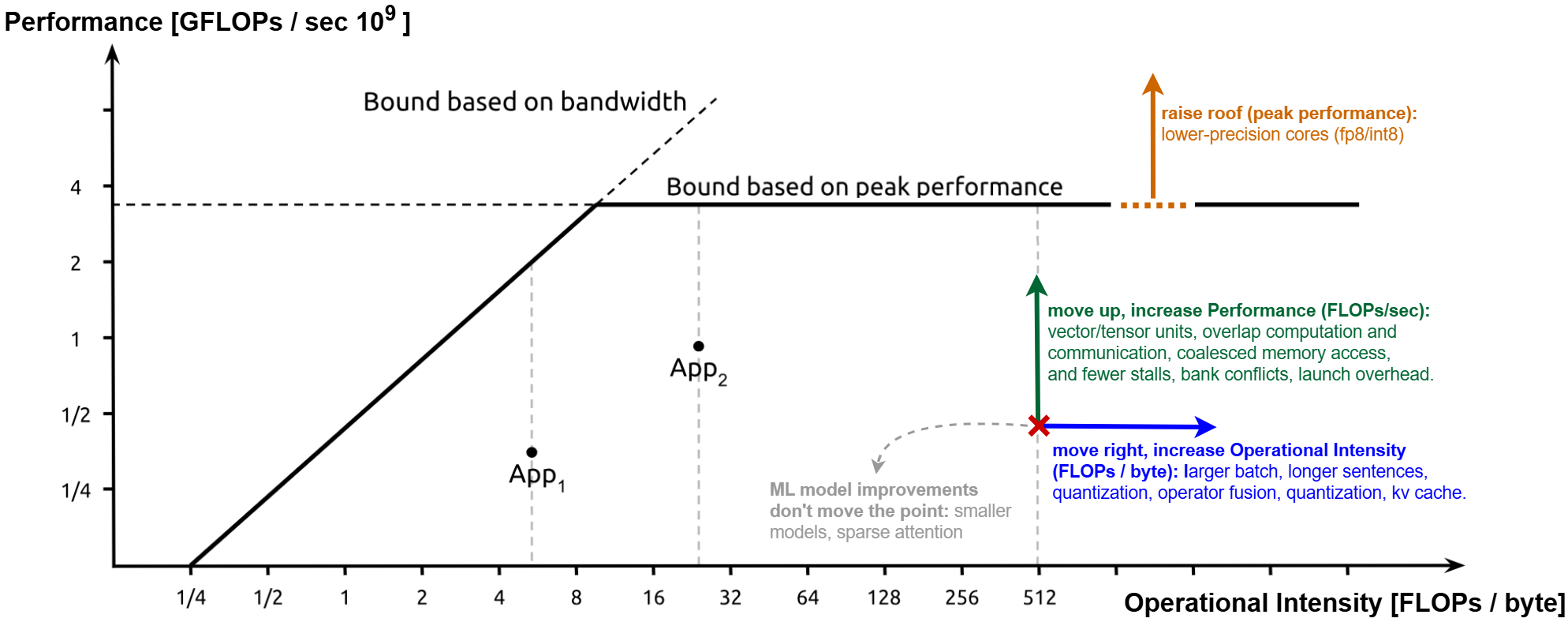
A roofline plot. App1 is memory-bound. App2 is compute-bound running below the peak performance. Adapted from Wikipedia’s Roofline Model.
On a log-log plot, the two terms of the minimum form a “roof”: a slanted line for the bandwidth bound, and a flat line for the peak compute, where they meet at the ridge point:
- Computation to the left of the ridge point is memory-bound: the processor waits for data, and the only ways to speed it up are to move fewer bytes or to do more work per byte. This is typically where the decode step falls.
- Computation to the right is compute-bound: only faster math, or less of it, helps. The gap shows how much is lost to other overheads, such as kernel launches, memory latencies or poor memory access patterns. This relates mostly to the prefill step, that is typically near to the roof line.
We can move a point right, by providing more FLOPs per byte, via:
- A larger batch or more tokens per pass, so each weight byte is reused across more rows. For decode, this means batching and speculative decoding, which verifies several draft tokens in one pass.
- Better data reuse through tiling and blocking in shared memory or SRAM.
- Operator fusion, which avoids writing intermediates out to DRAM and reading them back.
- Fewer bytes per FLOP: quantized weights and KV cache, and attention variants that shrink the KV cache (GQA, MLA). These matter most for decode, which is dominated by weight and KV-cache reads.
We can move a point up, i.e. closer to the roof at the same intensity, by:
- Using tensor cores or matrix units and vectorized instructions.
- Good occupancy and overlapping compute with memory transfers.
- Coalesced, aligned memory access, which brings achieved bandwidth closer to peak.
- Fewer stalls: synchronization, bank conflicts, warp divergence, and kernel launch overhead (reduced with CUDA graphs, which helps decode’s many small kernels).
For compute-bound prefill, which is already near the flat roof, the remaining gains come from:
- Raising the roof: lower-precision tensor-core math such as FP8 or FP4.
- Doing less work: sparse attention or smaller models. These cut runtime without necessarily moving the point on the plot.
How to calculate the roofline point for an application
To find the \(X\) coordinate of our application (❌ in the roofline plot above), we need to find the total count of floating-point operations relative to data throughput, eg by looking at our code or using hardware counters:
\[\text{Arithmetic Intensity } (X) = \frac{\text{Total FLOPs executed}}{\text{Total Bytes read and written}}\]To find the \(Y\) coordinate of ❌, we measure the execution wall-clock time of the specific kernel:
\[\text{Performance } (Y) = \frac{\text{Total FLOPs executed}}{\text{Execution Time (Seconds)} \times 10^9} \quad \text{[GFLOPs/s]}\]Vector Sum (real use case)
Consider a vector loop processing \(N = 1,000,000\) elements calculating \(C[i] = A[i] + B[i]\) using 32-bit single-precision floats (\(1 \text{ float} = 4 \text{ bytes}\)).
- Total FLOPs: 1 addition per iteration \(\times 1,000,000 = 1,000,000 \text{ FLOPs}\).
- Total Bytes: Read array \(A\) (\(4\text{MB}\)), read array \(B\) (\(4\text{MB}\)), write array \(C\) (\(4\text{MB}\)) = \(12,000,000 \text{ bytes}\).
- \(X\) Coordinate: \(1,000,000 / 12,000,000 = \mathbf{0.083 \text{ FLOPs/byte}}\).
If the GPU runs the vector loop above in exactly \(0.0001 \text{ seconds}\):
- \(Y\) Coordinate: \(1,000,000 / (0.0001 \times 10^9) = \mathbf{10 \text{ GFLOPs/s}}\).
Therefore the roofline points ❌ for this example is \(\mathbf{(0.083, 10)}\).
Matrix Multiplication (general formulation)
For a matrix multiplication of two matrices with shapes \(A \times B\) and \(B \times C\), resulting in an output matrix of shape \(A \times C\), here are the FLOPs and memory traffic calculations, for a data type size of \(dt\) bytes per element.
Step 1: Floating Point Operations (FLOPs). To compute each of the \(AC\) elements in the output matrix, you perform a dot product consisting of \(B\) multiplications and \(B\) additions. Each multiply-accumulate counts as \(2\) FLOPs. Therefore:
\[\text{Total FLOPs} = 2ABC\]Step 2, naive: Memory Traffic (Bytes) for an implementation without cache. The number of bytes loaded from memory depends heavily on the implementation algorithm (naive vs. tiled/optimized). If every element is fetched directly from main memory without utilizing cache reuse:
- Matrix 1 (\(AB\)) loaded \(C\) times (once for every column in Matrix 2). \(\text{Bytes} = ABC\text{ }dt\)
- Matrix 2 (\(BC\)) loaded \(A\) times (once for every row in Matrix 1). \(\text{Bytes} = ABC\text{ }dt\)
- Total Bytes loaded: \(2ABC\text{ }dt\) bytes.
Step 2, cache-optimized: Memory Traffic (Bytes) for an implementation with cache. In hardware-accelerated environments (like GPUs using shared memory/tiling or Tensor Cores), data is loaded into fast on-chip SRAM/cache and reused across multiple calculations:
- Matrix 1 loaded \(AB\text{ }dt\) bytes (each element loaded once).
- Matrix 2 loaded \(BC\text{ }dt\) bytes (each element loaded once).
- Output Written: \(AC\text{ }dt\) bytes.
- Total Memory Traffic (loaded + written): \((AB + BC + AC)\text{ }dt \text{ bytes}\)
Step 3: Arithmetic Intensity (Operational Intensity). Dividing the total FLOPs by the minimum memory traffic gives the arithmetic intensity (FLOPs per byte transferred):
\[\text{Arithmetic Intensity} = \frac{2ABC}{(AB + BC + AC)\text{ }dt}\]For large square matrices where \(A = B = C = N\), this simplifies to roughly \(\frac{2N}{3\text{ }dt}\) FLOPs per byte, making matrix multiplication compute-bound for large sizes and memory-bound for very small sizes.
Step 4: Achieved Performance and Roofline Coordinate. To plot the point ❌ on the Roofline model, we combine the arithmetic intensity (X-axis) with the achieved performance in GFLOPs per second (Y-axis). The Y-axis value (Performance) is given by:
\[\text{Performance (GFLOPs/s)} = \frac{\text{Total FLOPs}}{\text{Execution Time (seconds)} \times 10^9} = \frac{2ABC}{\text{Time}_{\text{sec}} \times 10^9}\]leading to the final roofline coordinate ❌:
\[(X, Y) = \left( \frac{2ABC}{(AB + BC + AC)\text{ }dt} \; \frac{2ABC}{\text{Time}_{\text{sec}} \times 10^9} \right)\]Tensor multiplication
When expanding matrix multiplication to higher-dimensional tensors with e.g. shapes \(A \times B \times D \times E \times F\) and \(B \times C \times D \times E \times F\), the extra dimensions (\(D \times E \times F\)) act as batch or parallel execution axes. Both the total FLOPs and the memory traffic scale up by this batch size factor, which means it completely cancels out in the arithmetic intensity equation—leaving your X-axis coordinate identical to the standard 2D case.
However, because the total workload increases, the Y-axis performance scales up proportionally by the batch size \(DEF\), resulting in the final Roofline coordinate:
\[(X, Y) = \left( \frac{2ABC}{(AB + BC + AC) \text{ } dt} \; \frac{2ABC \text{ } DEF}{\text{Time}_{\text{sec}} \times 10^9} \right)\]Side note: FLOPs on forward and reverse passes
(heavily based on the scaling book)
In the context of model training, the primary objective shifts from simply generating a forward-pass output to also computing gradients in the backward pass. Consider a layer where input \(X\) (dimensions \(A \times B\)) multiplies by weights \(W\) (dimensions \(B \times C\)) to yield \(Y = XW\) (dimensions \(A \times C\)). Applying the chain rule, the gradient of the loss \(L\) with respect to the weight matrix \(W\) is:
\[\frac{\partial L}{\partial W} = X^T \left(\frac{\partial L}{\partial Y}\right)\]At its core, calculating that gradient involves a standard matrix multiplication. Even though it has calculus notation (∂), the actual operation your computer performs is multiplying a matrix by another matrix—in this example, \(X^T\) times the incoming gradient. So it costs approximately the same number of FLOPs as any other matrix multiplication of those dimensions. Here it requires approximately \(2ABC\) FLOPs, contracting over the \(A\) dimension. Similarly, the gradient with respect to the input \(X\) is:
\[\frac{\partial L}{\partial X} = \left(\frac{\partial L}{\partial Y}\right) W^T\]This also totals approximately \(2ABC\) FLOPs, given that \(\frac{\partial L}{\partial Y}\) has dimensions \(A \times C\). Therefore, when both gradients are needed, the backward pass requires about twice the FLOPs of the forward pass: it computes gradients with respect to the weights and the input. The incoming gradient \(\frac{\partial L}{\partial Y}\) is supplied by the next layer (or computed from the loss for the final layer).
In brief, this layer requires approximately \(2ABC\) FLOPs for the forward pass (and inference) and \(4ABC\) FLOPs for the backward pass, for a total of \(6ABC\) FLOPs for a full training step. For a transformer linear layer, if \(BC\) is the number of weights and \(A\) is the number of tokens processed, this is approximately \(6 \times \text{number of weights} \times \text{number of tokens}\) FLOPs, or \(6 \times \text{number of weights}\) FLOPs per token. This estimate covers the matrix multiplications and omits other operations.
Finally, for a weight matrix \(W\) with \(B \times C\) parameters, the optimizer update step (including updating the model parameters) for the Stochastic Gradient Descent computes:
\[W \leftarrow W-\eta g\]for learning rate \(\eta\) and gradients \(g\), and requires \(2BC\) FLOPs, due to one multiplication and one subtraction per parameter.
How to draw the Roofline for a GPU Architecture
To sketch out the limits of a hardware architecture, we need two values from the manufacturer’s specification sheet (for your chosen precision level, e.g., FP32):
- Peak Compute Performance (\(P_{\text{peak}}\)): Measured in GFLOPs/s.
- Peak Memory Bandwidth (\(B_{\text{peak}}\)): Measured in GB/s.
The Ridge Point is the architectural inflection point where the hardware shifts from being purely memory-bound to purely compute-bound.
\[\text{Ridge Point} = \frac{\text{Peak Compute Performance } (P_{\text{peak}})}{\text{Peak Memory Bandwidth } (B_{\text{peak}})}\]- Example (NVIDIA A100 PCIe FP32): \(P_{\text{peak}} = 19,500 \text{ GFLOPs/s}\) and \(B_{\text{peak}} = 1,555 \text{ GB/s}\).
- \(\text{Ridge Point} = 19,500 / 1,555 \approx \mathbf{12.54 \text{ FLOPs/byte}}\).
The draw Roodline model lines, we use a Logarithmic scale on both dimensions:
- The Sloped Line (Left Side) where \(x < \text{Ridge Point}\) is drawn by a 45-degree straight diagonal line - this is our memory ceiling.
- The The Horizontal Line (Right Side) is a completely flat, horizontal line from \(x \ge \text{Ridge Point}\) - this represents the Compute Ceiling.
The following code generates the roofline model for a given hardware and operation.
Show code
import matplotlib.pyplot as plt
import numpy as np

# 1. HARDWARE SPECS (e.g., NVIDIA A100 GPU)
P_peak = 19500  # Peak Compute: 19,500 GFLOPs/s
B_peak = 1555   # Peak Bandwidth: 1,555 GB/s
ridge_point = P_peak / B_peak  # ~12.54 FLOPs/byte

# 2. CODE SPECS (Vector Addition Example)
total_flops = 1_000_000                  # 1M additions
total_bytes = 1_000_000 * 3 * 4          # 3 arrays (A,B,C) of 4-byte floats
code_x = total_flops / total_bytes       # Arithmetic Intensity = FLOPs / Bytes = 0.083

# Performance = FLOPs / (Time * 1e9)
execution_time = 0.0001                  # 0.1 milliseconds
code_y = total_flops / (execution_time * 1e9)  # 10 GFLOPs/s

# 3. GENERATE ROOFLINE BOUNDARIES
x_line = np.logspace(-2, 3, 500)
y_line = np.minimum(P_peak, B_peak * x_line)

# 4. PLOT THE CHART
plt.figure(figsize=(8, 5))
plt.loglog(x_line, y_line, label="GPU Roofline Boundary", color="red", lw=2)
plt.scatter([code_x], [code_y], color="blue", s=100, zorder=5, label="Your Code")
plt.text(ridge_point * 1.2, P_peak * 0.7, f"Ridge Point: {ridge_point:.2f} FLOPs/B", color="red")
plt.text(code_x * 1.2, code_y, f"Your Code ({code_x:.3f}, {code_y:.1f})", color="blue")
plt.xlabel("Arithmetic Intensity (FLOPs/byte)")
plt.ylabel("Attainable Performance (GFLOPs/s)")
plt.title("Simple GPU Roofline Model Analysis")
plt.grid(True, which="both", ls="--")
plt.legend()
plt.savefig("simple_roofline.png") # Save the plot
plt.show()
Caching
There are three kinds of inference caching, each operating at a different layer of the stack (this three-layer view is adapted from this guide):
- KV caching stores the attention keys and values computed during a single request, so that the model does not recompute them at every decode step. Every serving engine uses it.
- Prefix caching extends KV caching across requests. When different requests share the same leading tokens, such as a system prompt, a reference document, few-shot examples or the previous turns of a conversation, the keys and values of that shared prefix are computed once and reused. It is also called prompt caching or context caching.
- Semantic caching is an application-level cache that stores complete input/output pairs and retrieves them by meaning. Unlike prefix caching, which reuses internal attention states, semantic caching skips the model call entirely when a sufficiently similar query was answered before.
These are complementary layers, not alternatives. KV caching is always on, prefix caching is the highest-leverage optimization for most production applications, and semantic caching pays off when many queries are similar. In short: the KV cache reuses work within one generation, prefix caching reuses work across requests, and semantic caching reuses whole answers.
KV cache
In the attention layer, the query of the new token attends to the keys and values of all previous tokens. In a causal model, the keys and values of past tokens never change, since token \(i\) only depends on the tokens before it. Without a cache, each decode step recomputes the keys and values of the whole sequence, so generating \(n\) tokens costs \(O(n^2)\) work in the projections and MLPs and \(O(n^3)\) in attention. With a cache, each step only computes the query, key and value of the new token, appends the new key and value to the cache, and attends over all cached ones: \(O(n)\) and \(O(n^2)\) in total. Queries do not need to be cached, because the query of a past token was only needed to compute the output at that past position.
The price is memory. For every token, every layer stores a key and a value vector per key-value head:
\[\text{KV cache size} = 2 \times n_\text{layers} \times n_\text{kv heads} \times d_\text{head} \times \text{bytes per value} \times \text{sequence length} \times \text{batch size}\]This memory, not compute, often limits how many sequences can be batched together, which is why many techniques in this post shrink the KV cache.
Two implementation details matter in practice:
- A dynamic cache grows by concatenating the new keys and values to the cache at every step. This is simple, but every concatenation allocates a new tensor and copies the whole cache. A static cache preallocates a buffer for the maximum sequence length and writes each new entry in place.
- Many models use learned absolute positional embeddings and a context window of
seqlentokens. When a sequence grows longer thanseqlen, the model without a cache slides its window and re-encodes the lastseqlentokens at positions 0 toseqlen-1, at every step. A KV cache cannot reproduce this, because the cached keys and values were computed at their original positions and with the context available back then. The model with a cache therefore matches the original model exactly for the firstseqlentokens only.
The following code implements a KV cache in our GPTlite model. The full code is in gptlite_kvcache.py and main_kvcache.py (text generation with and without the cache).
- Our implementation keeps the last
seqlenkeys and values, and gives every new token the last position,seqlen-1: generation can continue past the context window, but its output no longer matches the original model. Models with relative positional encodings, such as RoPE, handle a sliding window more gracefully, but keeping only the most recent tokens still changes the output. - Our implementation also accepts several new tokens on top of a cache, which prefix caching and speculative decoding need: the causal mask is shifted, so that each new token attends to all the cached tokens and to the new ones up to itself.
Show code
# gptlite_kvcache.py: Sq new tokens attend to the cached keys and values, and to the new ones up to themselves
def scaled_dot_product_attention_kv_cache(Q, K, V, causal_mask=True, dropout=None):
    scores = torch.matmul(Q, K.transpose(-2, -1)) / (K.size(-1) ** 0.5)  # [B, H, Sq, Sk]
    Sq, Sk = Q.size(2), K.size(2)
    if causal_mask and Sq > 1:
        mask = torch.ones(Sq, Sk, device=Q.device).tril(diagonal=Sk - Sq)
        scores = scores.masked_fill(mask == 0, float('-inf'))
    # ...

class MultiHeadAttention_KVCache(nn.Module):

    def forward(self, x, kv_cache=None, causal_mask=True, max_seqlen=None):
        B, S, _ = x.shape
        H, D = self.n_heads, self.d_head

        # Compute Q, K, V of the new tokens
        q = self.query_proj(x).view(B, S, H, D).transpose(1, 2)  # [B, H, S, D]
        k = self.key_proj(x).view(B, S, H, D).transpose(1, 2)
        v = self.value_proj(x).view(B, S, H, D).transpose(1, 2)

        # If a cache is provided, prepend the past keys and values
        if kv_cache is not None:
            past_keys, past_values = kv_cache
            k = torch.cat([past_keys, k], dim=2)  # [B, H, S_past + S, D]
            v = torch.cat([past_values, v], dim=2)
            # Keep at most the last max_seqlen keys and values
            if max_seqlen is not None and k.size(2) > max_seqlen:
                k = k[:, :, -max_seqlen:, :]
                v = v[:, :, -max_seqlen:, :]

        out = scaled_dot_product_attention_kv_cache(q, k, v, causal_mask=causal_mask,
                                          dropout=self.dropout if self.training else None)
        # ...
        new_cache = (k, v)
        return out, new_cache

# gptlite_kvcache.py: the new tokens follow the cached ones
class GPTlite_KVCache(nn.Module):

    def forward(self, x, kv_cache=None, max_seqlen=None):
        B, T = x.shape
        if kv_cache is not None and kv_cache[0] is not None:
            S_past = kv_cache[0][0].size(2)  # S_past from first layer's past_keys
            positions = torch.arange(S_past, S_past + T, device=x.device).clamp(max=self.seqlen - 1)
            positions = positions.unsqueeze(0).expand(B, T)
        else:
            positions = torch.arange(T, device=x.device).unsqueeze(0).expand(B, T)
        # ...
        # Process through blocks: one cache per layer
        new_caches = []
        for block, layer_cache in zip(self.blocks, kv_cache):
            x, new_cache = block(x, kv_cache=layer_cache, max_seqlen=max_seqlen)
            new_caches.append(new_cache)
        # ...
        return x, new_caches

# main_kvcache.py: process the prompt once (prefill), then one new token per step (decode)
def generate_kvcache(model, prompt, n_tokens, seqlen, kv_cache=None):
  logits, kv_cache = model(prompt, kv_cache=kv_cache, max_seqlen=seqlen)
  tokens = prompt
  for i in range(n_tokens):
    next_token = torch.argmax(logits[:, -1], dim=-1, keepdim=True)
    tokens = torch.cat([tokens, next_token], dim=-1)
    if i < n_tokens - 1:
      logits, kv_cache = model(next_token, kv_cache=kv_cache, max_seqlen=seqlen)
  return tokens
PagedAttention: memory management for the KV cache
Continuous batching makes memory management hard, because the final length of each sequence is unknown. A naive engine reserves a contiguous KV buffer of the maximum length for every request, and most of that memory stays empty: the authors of vLLM measured that only 20% to 40% of the KV memory reserved by existing systems held actual tokens. PagedAttention borrows the idea of virtual memory from operating systems. The KV cache is split into fixed-size blocks (pages) that are allocated on demand, and a block table maps the logical blocks of each sequence to physical blocks anywhere in GPU memory. The attention kernel reads the blocks through this table. Almost no memory is wasted, so more sequences fit in a batch: vLLM reported 2-4 times higher throughput than previous systems. Blocks can also be shared by several sequences and copied only when one of them writes to it (copy-on-write), which is how prefix caching, parallel sampling and beam search share their common prefix. The code can be found in The full code is in paged_attention.py
Prefix caching, prompt caching or context caching
Many requests start with the same tokens: a system prompt, tool definitions, a long document that users ask several questions about, or the history of a conversation. Prefix caching keeps the keys and values of these tokens after a request finishes, so that the next request starting with the same tokens skips their prefill and only processes its new part. The first token arrives much sooner, and the GPU is free for other work.
How the lookup works. vLLM splits KV cache into fixed-size blocks (e.g., 16 tokens) and identifies each block by a hash of its tokens combined with the hash of the previous block. The chain of hashes identifies the whole prefix, so a lookup walks the blocks from the start of the prompt and stops at the first miss.
- During the request: prefill computes the K/V of all P prompt tokens in one pass, and each decode step appends the K/V of one new token. At the end the cache holds all prefill and decode tokens.
- Labeling: each full block gets a hash of its 16 token IDs combined with the previous block’s hash. So a block’s hash identifies the whole prefix up to the end of that block.
- Next request: the engine hashes the new tokens block by block from the start, reuses blocks until the first mismatch, and only prefills the rest.
Automatic Prefix Caching does not require extra memory storage. It operates almost entirely by reusing existing memory spaces using pointers. Because vLLM is built natively on PagedAttention, memory is already divided into discrete, fixed-size physical memory pages (blocks of tokens, usually 16 tokens per block). Prefix caching simply piggybacks off this virtual memory architecture.
SGLang’s RadixAttention stores all cached sequences in a radix tree (a compressed prefix tree), finds the longest prefix shared with each new request, and evicts the least recently used leaves when memory runs out.
Why the prefix must match exactly. It is tempting to look for similar prompts, e.g., with a vector database, instead of identical ones. This does not work for attention states. The key and value of token \(i\) depend on all the tokens before it, through every layer of the model. Two prompts that differ in a single early token, even if they mean the same, have different keys and values for every token after that difference. Reusing the cache of a similar prompt would silently feed the model a different context than the one the user sent. Exact matching makes prefix caching lossless: the output is identical to running the model without the cache. It is also cheap: a hash or tree lookup, instead of computing an embedding and searching a vector index. Similarity search does make sense one level up, where whole answers are reused: that is semantic caching, below.
Prefixes, not substrings. For the same reason, only a prefix can be reused, i.e., the first \(N\) tokens of the prompt. A paragraph in the middle of a prompt has different keys and values depending on what comes before it. Matching is done on token IDs, not on raw text, so the same text tokenized differently (e.g., with an extra space) is a miss. Research systems reuse non-prefix chunks approximately: CacheBlend precomputes the cache of each retrieved document independently and recomputes a small fraction of tokens to restore the attention between documents, and Prompt Cache reuses precomputed modules of prompts written in a structured template.
What is kept. The KV cache holds the keys and values of every token processed so far, in every layer: the prompt and all the generated tokens, not only the last decode step, since every new token attends to all of them. When a request finishes, its blocks are not freed right away: they stay in memory, marked as reusable, until the memory is needed for something else. Generated tokens are cached too, which is what makes multi-turn chat fast: the prompt of the next turn is the previous prompt, plus the previous answer, plus the new message. Thus, we put the static content first (system prompt, tools, documents) on the query, and the variable content last (the user’s question, timestamps): anything that changes early in the prompt invalidates the cache for everything after it.
The following code implements prefix caching on top of the KV cache: the keys and values of a shared prefix are computed once, and reused by every request. The full code is in main_prefix_cache.py, which also checks that the outputs are the same as without prefix caching:
Show code
# without prefix caching: every request processes the shared prefix again
for request in requests:
  generate_kvcache(model, torch.cat([prefix, request[None]], dim=1), n_tokens, seqlen)

# with prefix caching: the keys and values of the prefix are computed once and reused by every
# request. Attention creates new tensors when it appends to the cache (torch.cat), so the prefix
# cache is never modified and can be shared by all requests
_, prefix_cache = model(prefix)
for request in requests:
  generate_kvcache(model, request[None], n_tokens, seqlen, kv_cache=prefix_cache)
Semantic caching
A semantic cache sits in front of the model, in the application. For every incoming query, it:
- computes an embedding, a vector that represents the meaning of the query;
- searches a vector index for the most similar past query;
- if the similarity is above a threshold, returns the stored answer without calling the model;
- otherwise, calls the model and stores the new (embedding, answer) pair.
How embeddings are created. Embeddings come from a separate and much smaller embedding model, typically a transformer encoder such as the Sentence-BERT family (e.g., all-MiniLM-L6-v2), E5, BGE or GTE, or from an embedding API. The encoder is trained with contrastive learning: pairs of texts with the same meaning (paraphrases, or a question and its answer) are pulled together, and the other texts of the batch are pushed apart. After training, the cosine similarity between two embeddings measures how close their meanings are. The raw hidden states of a generative LLM make poor embeddings unless the model is fine-tuned in the same contrastive way, which is how some of the best recent embedding models are built.
Where embeddings are stored. Any vector database/index works. FAISS is a popular choice: an in-process library, for CPUs and GPUs, with exact indexes (e.g., IndexFlatIP, an inner product, which equals the cosine similarity for normalized vectors) and approximate ones for millions of vectors (IVF, HNSW, product quantization). Since FAISS is a library and not a database, persistence, metadata, deletions and expiration are up to us; vector databases such as Milvus, Qdrant, Weaviate, pgvector or Redis provide them. Tools such as GPTCache implement the whole loop and support FAISS as a backend.
Risks. A semantic cache is approximate, so it can return a wrong answer: “how do I delete a file in Python?” and “how do I delete a folder in Python?” are very similar sentences with different answers. Answers also go stale, and queries that depend on the conversation history or on the user should not share answers. In practice, we tune the threshold on real traffic, scope the cache per user or tenant, add an expiration time, and optionally confirm hits with a more precise re-ranking model. The strict version of a semantic cache is the exact-match cache, which maps a hash of the full request (prompt, model and sampling parameters) to the response. It never returns a wrong answer, but only hits identical requests.
The following code implements a minimal semantic cache with FAISS and a pre-trained sentence encoder. GPTlite is a character-level model trained on Shakespeare, so it cannot answer questions: here, it is only a stand-in for the LLM behind the cache. The full code is in main_semantic_cache.py, which prints the similarity of each query to the closest cached one, to help choose the threshold:
Show code
class SemanticCache:
  """ Cache of (query, answer) pairs, looked up by the cosine similarity of the query embeddings """

  def __init__(self, embed_fn, threshold):
    self.embed_fn = embed_fn  # maps a list of strings to unit-norm float32 embeddings of shape [n, dim]
    dim = embed_fn(["probe"]).shape[1]
    self.index = faiss.IndexFlatIP(dim)  # exact search, inner product = cosine similarity of unit vectors
    self.answers = []
    self.threshold = threshold

  def __call__(self, query, generate_fn):
    """ Returns the answer to the query, the similarity to the closest cached query, and if it was a hit """
    embedding = self.embed_fn([query])
    similarity = 0.0
    if self.index.ntotal > 0:
      similarities, ids = self.index.search(embedding, 1)  # most similar cached query
      similarity = float(similarities[0, 0])
      if similarity >= self.threshold:
        return self.answers[ids[0, 0]], similarity, True
    answer = generate_fn(query)  # cache miss: call the model and store the new pair
    self.index.add(embedding)
    self.answers.append(answer)
    return answer, similarity, False

def sentence_transformer_embedder(model_name="all-MiniLM-L6-v2"):
  """ Embedding function of a pre-trained sentence encoder (downloaded on first use) """
  from sentence_transformers import SentenceTransformer
  encoder = SentenceTransformer(model_name)
  return lambda texts: encoder.encode(texts, normalize_embeddings=True).astype(np.float32)

# usage
cache = SemanticCache(sentence_transformer_embedder(), threshold=0.85)
answer, similarity, hit = cache(query, generate_fn)
Batching improvements
Batching is the most effective way to increase throughput. Because decode is memory-bound, a decode step for a batch of 32 sequences takes almost the same time as for a single sequence: the weights are read once and used 32 times. Throughput grows almost linearly with the batch size, until the GPU becomes compute-bound or runs out of memory for the KV caches. The difficulty is that requests arrive at different times and generate different numbers of tokens.
The simplest approach groups \(B\) requests and runs them together until all of them finish. Sequences that finish early keep their slot and generate tokens that are thrown away, and new requests wait until the whole batch is done. Prompts of different lengths are padded to the same length. We pad on the right: with causal attention, real tokens never attend to the padding that follows them, so no attention mask is needed, and each sequence reads its next-token prediction at its own last position. Padding on the left would require a padding mask and shifted positions instead. This static batching is not ideal as it requires unnecessary computation and memory for the padded indices.
Continuous batching, introduced by Orca as iteration-level scheduling, takes the scheduling decision at every decode step instead of once per batch: as soon as a sequence finishes, it leaves the batch, and a waiting request takes its slot. The GPU stays busy, and new requests do not wait for the longest sequence of the previous batch. The implementation must track each sequence separately, by keeping the tokens of every running request apart, and rebuilds the right-padded batch at every step, so a new request never sees the tokens of the previous occupant of its slot.
Ragged/packed batching. A GPU may hold prefill and decode steps from different samples in the same compute step. Engines don’t pad sequences into a rectangle ie into a batch otherwise sentences of different length would require substantial padding. Instead, queries are concatenated and each step is one forward pass over a flat list of tokens from all running sequences. The next token predicted by each query will be placed on \(i+1\) of the output tensor, where \(i\) is the last index of the input query. This is ragged/packed batching:
- Linear layers: the MLP and the projections don’t care which sequence a token belongs to, so they run as one large matrix multiplication over all the step’s tokens.
- Attention: only attention is per sequence. Variable-length kernels (FlashAttention’s varlen mode, FlashInfer, PagedAttention) use per-token metadata (sequence id, position, KV block table) so each token attends only to its own sequence. To separate sentences, Instead of a dense, wasteful square matrix, the attention is handled using a Block-Diagonal Attention Mask.
- When the forward pass hits the final Softmax layer, it doesn’t compute predictions for every position. It looks up the metadata map, isolates the exact indices that represent the final token of each request (the end boundaries), and performs the argmax/sampling logic only on those token slices to extract the next token for every active query.
Mixing prefill and decode to improve performance. This is the roofline picture again. Decode tokens alone are memory-bound and leave most GPU’s compute idle. But adding prefill chunks to the same step means many more tokens share each weight read, which pushes the step toward the ridge point - this is why Sarathi-Serve calls “stall-free batching”. To further improve GPU utilization:
- Dynamic scheduling. At every step the scheduler decides which requests run, how many tokens each contributes, which waiting requests to admit, and whom to preempt. These decisions are bounded by the token budget and by the free KV cache blocks.
- Token budget. The scheduler assigns each step a fixed number of tokens. It adds every decode first, to keep time per token low, and then fills the rest with prefill chunks.
- Reducing CPU overhead is done by doing CUDA graphs for decode-only steps, and scheduling the next step on the CPU while the GPU runs the current one (as SGLang does).
- Chunked prefill means processing a long prompt in several smaller pieces instead of in one forward pass. Each chunk, say 512 tokens, attends to the KV cache of the earlier chunks.Say an 8,000-token prompt arrives while 50 other sequences are decoding:
- Without chunking: one step must process all 8,000 prompt tokens plus the 50 decode tokens. That step takes far longer than a normal decode step, so all 50 users see their text pause.
- With chunking and a budget of 512 tokens per step: each step processes the 50 decode tokens plus 462 prompt tokens. The prompt finishes in about 18 steps, and the other users never notice.
- Note: because attention is causal, the result of is identical to processing the whole prompt at once. In practice, it works by progressively accumulating the Key-Value (KV) cache chunk-by-chunk and utilizes FlashAttention-style mechanics to calculate the partial attention math correctly.
- If we have a causal mask, tokens only need to attend to previous tokens, therefore attention is final after each chunk. If mask is not causal, it requires a final extra computation over the attention of previous chunks. This recomputational cost step requires reloading previous chunks back into GPU SRAM, increasing memory bandwidth overhead. For that reason, chunked prefill is rarely used for non-causal models.
Memory pressure. The KV cache is the real limit.
- Admission: a request is admitted only if enough free blocks exist.
- Preemption: if running sequences outgrow the cache, the scheduler evicts one, usually the newest. It then either drops its KV and recomputes it later (vLLM’s approach) or swaps its blocks to CPU memory.
- More capacity: FP8 KV cache, offloading, and evicting old prefix-cache blocks stretch the available memory.

Source: redhat post Meet vLLM: For faster, more efficient LLM inference and serving
Code. The following code implements continuous batching. The full code is in main_continuous_batching.py, which runs static and continuous batching on the same requests: both produce the same outputs, but continuous batching needs fewer steps, since its slots spend more time generating useful tokens:
Show code
def continuous_batching(model, requests, batch_size, seqlen):
  """ Keeps batch_size slots busy: as soon as a request finishes, the next waiting request takes its slot """
  outputs, n_steps = [None] * len(requests), 0
  waiting = list(range(len(requests)))  # ids of the requests waiting for a slot
  running = []  # (request id, tokens so far) of the requests in the batch
  while waiting or running:
    while waiting and len(running) < batch_size:  # fill the free slots
      request_id = waiting.pop(0)
      running.append((request_id, requests[request_id][0]))
    tokens = next_tokens(model, [seq for _, seq in running], seqlen)
    running = [(request_id, torch.cat([seq, token[None]])) for (request_id, seq), token in zip(running, tokens)]
    n_steps += 1
    still_running = []
    for request_id, seq in running:  # finished requests leave the batch
      prompt, n_tokens = requests[request_id]
      if len(seq) == len(prompt) + n_tokens:
        outputs[request_id] = seq
      else:
        still_running.append((request_id, seq))
    running = still_running
  return outputs, n_steps
Prefill-decode disaggregation
Prefill is compute-bound and decode is memory-bound, so they interfere when they share GPUs, and each would prefer a different batch size and parallelism. Disaggregated serving runs them on separate pools of GPUs: prefill workers compute the KV cache of each prompt and send it over a fast interconnect to decode workers, which generate the answer. Each pool is sized and tuned for its own latency target: TTFT for prefill, TPOT for decode. This is the design of DistServe, Splitwise and Mooncake, the serving platform of Moonshot AI’s Kimi, and it is supported by open-source stacks such as NVIDIA Dynamo and llm-d.
The Core Issue: The KV Cache Handoff Bottleneck. If a decode step falls on a separate NPU that lacks the KV cache, the model cannot generate the next token. The NPU needs the entire history of Keys and Values up to that point. The system faces two choices:
- Recomputation (The CPU/NPU Burden): The decode NPU could recompute the prompt itself to rebuild the KV cache. However, this completely defeats the purpose of disaggregation, burning massive compute resources and spiking latency.
- Network Serialization (The Bandwidth Burden): The prefill NPU must serialize the multi-gigabyte KV cache tensor and send it over the network to the decode NPU.
Prefill-decode disaggregation require KV cache to be transmitted between prefill and decode nodes. To avoid sending and waiting for large KV cache chunks, modern engines use Layer-Wise Streaming (a pipeline overlap of computation and communication): as Layer 1 finishes its prefill, it immediately starts transmitting its KV cache chunks over the network while Layer 2 is still computing. The destination can be a NPU’s High-Bandwidth Memory (HBM), or in more advanced cases, a shared cluster acting as KV Cache Store e.g., Mooncake or LMCache.