Linear Regression and Matrix Factorization
The following sections detail closed-form solutions for two problems. Linear regression predicts an output from the features of an input, and its least squares and ridge regression solutions have a closed form. Matrix factorization predicts the missing values of a matrix, such as the ratings of a recommender system, and its alternating least squares solves each step in closed form.
Linear Regression
Regression relates an input variable to an output, either to predict new outputs or to understand the effect of the input on the output. A regression dataset consists of a set of \(N\) pairs \((x_n, y_n)\), with an input \(x_n\) of \(D\) features and an output (or label) \(y_n\). The goal of regression is to find a function \(f\) such that \(y_n \approx f(x_n)\), which then predicts the output of a new input. Fitting a multidimensional plane to the dataset means solving the (multiple) linear regression problem, by finding the weights \(w\) such that:
\[y_n \approx f(x_n) = w_0 + w_1 x_{n1} + ... + w_D x_{nD} \hspace{1cm}\text{, or simply}\hspace{1cm} y \approx f(X) = Xw.\]Here, \(w_0\) is the bias (or intercept), and the \(N \times (D+1)\) matrix \(X\) holds the inputs in its rows, after a first column of ones that multiplies \(w_0\).
An error or loss function \(L(w)\) indicates how good the estimation is. As an example, the Mean Squared Error (MSE) loss is defined as \(L(w) = \frac{1}{N} \sum_{n=1}^N [y_n - f(x_n)]^2\), and penalizes predictions with larger errors more heavily, due to the square term. Another loss function, the Mean Absolute Error (MAE), with \(L(w) = \frac{1}{N} \sum_{n=1}^N \vert y_n - f(x_n) \vert\), is more robust to outliers, as a model trained with the MSE is pulled much more strongly by them.
Least Squares
For the particular case of linear regression with the Mean Squared Error loss function, the problem is called Least Squares and has a closed-form solution, \(w = (X^TX)^{-1} X^Ty\), derived as follows. In practice, the following is minimized (the factor \(\frac{1}{N}\) does not change the minimum):
\[\begin{align*} \| y - Xw \|^2 = \, & (y-Xw)^T(y-Xw) \\ = \, & y^Ty - y^TXw - (Xw)^Ty + (Xw)^TXw \\ = \, & y^Ty - w^TX^Ty - w^TX^Ty + w^TX^TXw \\ = \, & y^Ty - 2 w^TX^Ty + w^TX^TXw\\ \end{align*}\]This requires computing the \(w\) that minimizes the loss or, equivalently (as the loss is a convex function of \(w\)), the \(w\) where its derivative is 0. So \(w\) is computed as:
\[\begin{align*} & \frac{\partial}{\partial w} \left( y^Ty - 2 w^TX^Ty + w^TX^TXw \right) = 0 \\ \Leftrightarrow \, & 0 - 2 X^Ty + 2 X^TXw = 0 \\ \Leftrightarrow \, & 2 X^TXw = 2X^Ty \\ \Leftrightarrow \, & w = (X^TX)^{-1} X^Ty\\ \end{align*}\]Note that the derivation used the trick \(\frac{\partial w^Ta}{\partial w} = \frac{\partial a^Tw}{\partial w} = a\) (The Matrix Cookbook, section 2.4.1, eq. 69) and \(\frac{\partial w^TAw}{\partial w} = (A + A^T)w\) (section 2.4.2, eq. 81). The third line of this derivation, once divided by 2, gives the normal equations \(X^TXw = X^Ty\). The result shows that if \(X^TX\) is invertible, this minimization problem has a unique closed-form solution, given by that final form.
As a side note, the Gram matrix \(X^TX\) is invertible if \(X\) has full column rank, i.e. \(\text{rank}(X)=D+1\), as its columns are the \(D\) inputs and the column of ones for the bias \(w_0\). Then, for any vector \(v\), \(X^TXv = 0\) implies \(\lVert Xv \rVert^2 = v^TX^TXv = 0\), i.e. \(Xv = 0\), which only holds for \(v = 0\), so \(X^TX\) is invertible.
In NumPy, the closed-form solution is written as in its formula, here for the three points \((0, 1)\), \((1, 2)\) and \((2, 4)\):
import numpy as np

X = np.array([[1, 0], [1, 1], [1, 2]])  # a column of ones, then the input of each point
y = np.array([1, 2, 4])
w = np.linalg.inv(X.T @ X) @ X.T @ y  # [0.833, 1.5]
In practice, libraries solve the normal equations without computing the inverse, which is faster and more accurate. The closed form takes \(O(ND^2 + D^3)\) operations, to compute \(X^TX\) and to invert it, so it suits problems with few features. For many features, the gradient descent of the post on algebra is used instead.
Regularization
It is common practice to add to the loss a regularization term \(\mathcal{R}(w)\) that penalizes complex models. Such models tend to fit the noise of the training data and to predict new data poorly, a problem called overfitting. The loss minimization problem then becomes:
\[\min_w L(w) + \mathcal{R}(w)\]Common regularization approaches are:
- L1 regularization: \(\mathcal{R}(w) = \lambda \lVert w \rVert_1\), where \(\lVert w \rVert_1 = \sum_{i=1}^D \vert w_i \vert\) (the bias \(w_0\) is not penalized). Linear regression with this term is called LASSO Regression, as in Least Absolute Shrinkage and Selection Operator;
- L2 regularization (standard Euclidean norm): \(\mathcal{R}(w) = \lambda \lVert w \rVert_2^2\), where \(\lVert w \rVert_2^2 = \sum_{i=1}^D w_i^2\). Large weights are penalized, as they are considered unlikely. If \(L\) is the MSE, this is called Ridge Regression.
In both, the parameter \(\lambda \gt 0\) can be tuned to reduce overfitting. This is the model selection problem.
LASSO encourages simple, sparse models (i.e. models with fewer parameters). This particular type of regression is well-suited to automate certain parts of model selection, like variable selection/parameter elimination. However, with highly correlated features (multicollinearity), LASSO tends to keep one of them arbitrarily, and Ridge Regression or the elastic net (L1 plus L2) are preferred.
Similarly to the Least Squares problem, the MSE loss with Ridge Regression has an analytical solution. It is computed by minimizing \((y - Xw)^T(y-Xw) + \lambda w^Tw\): differentiating with respect to \(w\) leads to the regularized normal equations \((X^TX + \lambda I)w = X^Ty\), with the solution \(w = (X^TX + \lambda I)^{-1} X^Ty\). This form also penalizes \(w_0\); excluding the bias sets the first diagonal entry of \(I\) to 0. The solution exists even when \(X^TX\) is not invertible, as \(v^T(X^TX + \lambda I)v = \lVert Xv \rVert^2 + \lambda \lVert v \rVert^2 > 0\) for any \(v \neq 0\), so \(X^TX + \lambda I\) is invertible. In code, Ridge Regression adds \(\lambda\) to the diagonal of \(X^TX\), except for the entry of the bias:
lam = 1.0
I = np.diag([0, 1])  # the bias w_0 is not penalized
w = np.linalg.inv(X.T @ X + lam * I) @ X.T @ y  # [1.333, 1.0]
Note: in statistics, shrinkage is the reduction in the effects of sampling variation on the estimated parameters (e.g. a model overfitting the training data and not performing well on unseen data). Regularization attempts to do this by “shrinking” model parameters towards 0: LASSO sets some of them exactly to 0, while Ridge Regression makes all of them smaller, without setting them to 0.
The difference shows on a single weight \(w\), whose loss \((w - \hat{w})^2\) has its minimum at the least squares value \(\hat{w}\). Minimizing \((w - \hat{w})^2 + \lambda \vert w \vert\) gives \(w = \text{sign}(\hat{w}) \max(\vert \hat{w} \vert - \lambda/2, 0)\), while minimizing \((w - \hat{w})^2 + \lambda w^2\) gives \(w = \hat{w}/(1 + \lambda)\). In practice, LASSO subtracts a constant from the magnitude of the weight and stops at 0, while Ridge Regression divides it by a constant and never reaches 0. The following picture illustrates the difference with two weights \(w_1\) and \(w_2\):
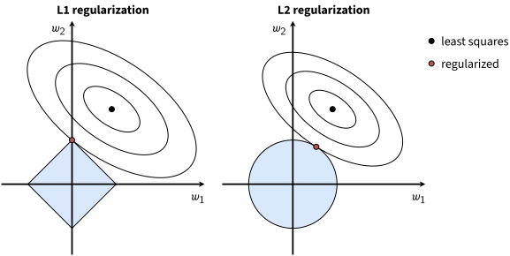
The contours of a squared loss (black ellipses) around its least squares solution, and the regions \(\lVert w \rVert_1 \le 1\) of L1 regularization (left) and \(\lVert w \rVert_2 \le 1\) of L2 regularization (right). Minimizing the regularized loss is equivalent to minimizing the loss inside such a region, of a size that depends on \(\lambda\): the solution is the point where the smallest contour touches the region, often a corner for L1 regularization, where a weight is 0.
Matrix Factorization
Matrix factorization can be used to discover underlying latent factors and/or to predict missing values of the matrix, as in recommender systems. The goal is to find \(W\) and \(Z\) such that \(X \approx WZ^T\), i.e. to predict \(x_{dn}\), where \(d\) indexes the rows of \(W\) and \(n\) the rows of \(Z\). For movie ratings, \(Z\) could be users, \(W\) could be movies, and \(x_{dn}\) the star rating. Each movie and each user is then described by a vector of \(K\) numbers, a row of \(W\) or of \(Z\), where \(K\) is the number of columns of both factors. The rating of a movie by a user is predicted by the dot product of their two vectors. Note that, in this section, \(X\) is the \(D \times N\) matrix of the ratings of \(D\) movies by \(N\) users, and no longer the data matrix of linear regression.
The aim is to optimize:
\[\min_{W,Z} L (W,Z) = \frac{1}{2} \sum_{(d,n) \in \Omega} [ x_{dn} - (WZ^T)_{dn}]^2\]where \(W \in \mathbb{R}^{D \times K}\) and \(Z \in \mathbb{R}^{N \times K}\) are tall matrices, and \(\Omega \subseteq [D] \times [N]\) collects the indices of the observed ratings of the input matrix \(X\). The following picture illustrates the factorization:
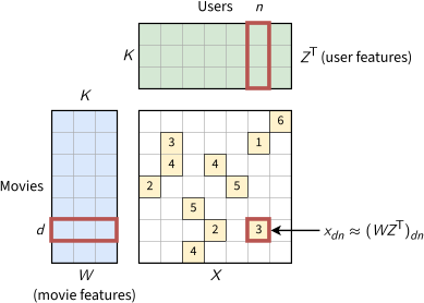
Matrix factorization \(X \approx WZ^T\) of the ratings of \(D = 7\) movies by \(N = 7\) users, with 11 observed ratings and \(K = 3\) latent features. The rating \(x_{dn}\) of movie \(d\) by user \(n\) is approximated by the dot product of row \(d\) of \(W\), the features of movie \(d\), and column \(n\) of \(Z^T\), the features of user \(n\).
This cost function is neither convex nor identifiable: for any invertible \(K \times K\) matrix \(Q\), the factors \(WQ\) and \(Z(Q^{-1})^T\) give the same product \(WZ^T\). \(K\) is the number of latent features (e.g. gender, age group, citizenship, etc.). A large \(K\) facilitates overfitting, as the factors hold \((D+N)K\) parameters. A regularizer can be added to the function:
\[\min_{W,Z} L (W,Z) = \frac{1}{2} \sum_{(d,n) \in \Omega} [ x_{dn} - (WZ^T)_{dn}]^2 + \frac{\lambda_w}{2} \| W \|^2 + \frac{\lambda_z}{2} \| Z \|^2\]where (again) \(\lambda_z\) and \(\lambda_w\) are scalars, and the norms are Frobenius norms. The cost can be minimized over one factor at a time, a form of coordinate descent.
Coordinate Descent
The coordinate descent optimization method iterates over individual coordinates (keeping the others fixed) to minimize the loss function, as illustrated below:
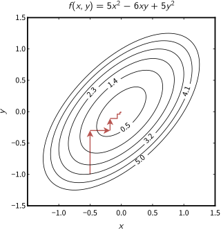
Coordinate descent on \(f(x, y) = 5x^2 - 6xy + 5y^2\) from \((-0.5, -1)\): each step minimizes \(f\) along one coordinate, alternating \(y\) and \(x\), and the iterates converge to the minimum at the origin. Adapted from: Coordinate descent
The main advantage is that it is extremely simple to implement and does not require any knowledge of the derivative of the function: the minimum along one coordinate can be found by a search along that coordinate (a line search). It is useful for extremely complicated functions or functions whose derivatives are far more expensive to compute than the function itself. However, due to its sequential nature, it is not a good candidate for parallelism, unless several coordinates can be minimized independently, as the rows of each factor in ALS, described next. Another issue arises with non-smooth multivariable functions: it may get stuck at a non-stationary point if the level curves of the function are not smooth.
Alternating Least Squares
Alternating Least Squares (ALS) factorizes the matrix \(X\) into the two factors \(W\) and \(Z\) such that \(X \approx WZ^T\), with a block coordinate descent. It minimizes the cost over all the entries of \(W\) for a fixed \(Z\), then over all the entries of \(Z\) for a fixed \(W\), and so on. With one factor fixed, the cost is quadratic in the other one, as in least squares, so each step has a closed-form solution and decreases the cost, until convergence:
-
If there are no missing ratings in the matrix, i.e. \(\Omega = [D] \times [N]\), then:
\[\begin{align*} \min_{W,Z} L(W,Z) = & \frac{1}{2} \sum_{d=1}^D \sum_{n=1}^N [x_{dn} - (WZ^T)_{dn}]^2 + \text{ (regularizer) } \\ = & \frac{1}{2} \| X - WZ^T \| ^2 + \frac{\lambda_w}{2} \| W \|^2 + \frac{\lambda_z}{2} \| Z \|^2 \end{align*}\]- the closed-form updates are \(W = XZ (Z^TZ + \lambda_w I_K)^{-1}\) for a fixed \(Z\), and \(Z = X^TW (W^TW + \lambda_z I_K)^{-1}\) for a fixed \(W\), where \(I_K\) is the \(K \times K\) identity matrix;
-
If there are missing entries, the problem is harder, as only the ratings \((d,n) \in \Omega\) contribute to the cost, i.e.:
\[\min_{W,Z} L(W,Z) = \frac{1}{2} \sum_{(d,n) \in \Omega} [x_{dn} - (WZ^T)_{dn}]^2 + ...\]- each row \(w_d\) of \(W\) is then computed from its observed ratings only, as \(w_d = (\sum_{n:(d,n) \in \Omega} z_n z_n^T + \lambda_w I_K)^{-1} \sum_{n:(d,n) \in \Omega} x_{dn} z_n\), and similarly for each row \(z_n\) of \(Z\).
Each step of ALS thus runs one Ridge Regression per row, of its observed ratings on the rows of the fixed factor. In code, mask is the \(D \times N\) boolean matrix of the observed ratings \(\Omega\), and the same \(\lambda\) is used for both factors. The function als_rows computes all the rows of one factor with the closed form above, and mf_als alternates between the two factors, from a random \(Z\):
def als_rows(F, X, mask, lam):
    """Each row of the other factor: a Ridge Regression of its observed ratings on F."""
    I = lam * np.eye(F.shape[1])
    return np.array([np.linalg.inv(F[m].T @ F[m] + I) @ F[m].T @ x[m] for x, m in zip(X, mask)])

def mf_als(X, mask, K, lam=0.1, iters=20):
    Z = np.random.default_rng(0).normal(0, 0.1, (X.shape[1], K))
    for _ in range(iters):
        W = als_rows(Z, X, mask, lam)  # each row w_d, for a fixed Z
        Z = als_rows(W, X.T, mask.T, lam)  # each row z_n, for a fixed W
    return W, Z
ALS is favorable in two cases (Koren et al., 2009). The first is parallel computing, as each row of \(W\) (or of \(Z\)) is computed independently of the other rows. The second is implicit feedback, such as purchases or views instead of ratings: the matrix then records whether each user bought or watched each item, so all its entries are known, and ALS handles such a dense matrix efficiently.