Mixture-of-Experts and Expert Parallelism
In a dense model, every parameter processes every token, and a forward pass takes about 2 FLOPs per parameter and token (one multiplication and one addition). A sparse Mixture-of-Experts (MoE) layer replaces a feed-forward network with \(N\) feed-forward networks, the experts, and a small router network that sends each token to only \(k\) of them. An MoE model is thus described by two numbers: its total parameters, which set its memory, and its active parameters, used for each token, which set its compute. Therefore, MoEs increase the model capacity per FLOP, which can improve scaling, efficiency and quality compared to dense models of a similar cost.
Early days: small MoEs as a weighted sum of expert outputs
In 1991, the papers Adaptive Mixtures of Local Experts and Task Decomposition Through Competition in a Modular Connectionist Architecture introduced some of the earliest architectures similar to what is now called an MoE. The following picture illustrates such an MoE (left), next to the deep MoE of the next section (right):
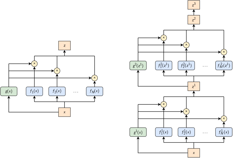
Adapted from: Learning Factored Representations in a Deep Mixture of Experts
The MoE was defined as a set of independent experts (feed-forward networks, \(f_i(x)\) in the picture) alongside a gating network (also a feed-forward network, \(g(x)\)). All the experts and the gating network receive the same input \(x\). The gating network outputs a distribution of each expert’s relevance/importance for the given input and can be defined in its simplest form with a softmax, as \(g(x) = \mathrm{Softmax}(x \cdot W_g)\), where \(W_g\) is a learnable transformation. Finally, the output of the system is the sum of the outputs of all experts weighted by the output of the gating network, \(z = \sum_i g_i(x) \, f_i(x)\), where \(g_i(x)\) is the gate value (the probability) of expert \(i\).
The implementation of an MoE module is straightforward. The router (the gating network) is a small feed-forward network that outputs, for every token, a probability per expert, and each expert is a regular feed-forward network. The input x holds \(B\) sequences of \(S\) tokens, each token an embedding of \(E\) elements (B*S*E in the comments of the code, where n_experts is the number of experts \(N\)):
class Router(nn.Module):
  """ a DNN to route tokens to experts """

  def __init__(self, n_embd, num_experts, dropout=0.1):
    super().__init__()
    self.net = nn.Sequential(
      nn.Dropout(dropout),
      nn.Linear(n_embd, n_embd*4), nn.ReLU(),
      nn.Linear(n_embd*4, n_embd*4), nn.ReLU(),
      nn.Linear(n_embd*4, num_experts), nn.Softmax(dim=-1)
    )

  def forward(self, x):
    return self.net(x)


class MoE(nn.Module):

  def __init__(self, input_size, output_size, num_experts, dropout=0.1):
    super().__init__()
    self.router = Router(input_size, num_experts, dropout=dropout)
    self.experts = nn.ModuleList([
      FeedForward(input_size, output_size, dropout=dropout) for _ in range(num_experts) ])

  def forward(self, x):
    probs = self.router(x)
    outputs = torch.stack([ expert(x) for expert in self.experts ], dim=-2) # B*S*n_experts*E
    weighted_outputs = outputs * probs.unsqueeze(-1) # B*S*n_experts*E x B*S*n_experts*1 -> B*S*n_experts*E
    weighted_sum = weighted_outputs.sum(dim=-2) # sum over experts: B*S*n_experts*E -> B*S*E
    return weighted_sum, probs, outputs
A major difference between the two 1991 approaches is the loss function. One uses the error function \(L = \lVert d - \sum_i g_i(x) \, f_i(x) \rVert^2\), the squared error of the output \(z\), where \(f_i(x)\) is the output vector of expert \(i\), \(g_i(x)\) is the router’s probability for expert \(i\), and \(d\) is the correct label for the input.
The other argues that this form makes the experts cooperate: each expert must cancel the residual error left by the others, so many experts are used for each input. It suggests instead the error function \(L = \sum_i g_i(x) \lVert d - f_i(x) \rVert^2\) (and variants based on the negative log-likelihood), in which each expert produces the whole output, so that the experts compete and a single expert tends to be used for each input.
As an example, take two experts with the same gate value, whose outputs miss the target by the same amount in opposite directions. Their errors cancel each other in the first error function, which is then zero, so neither expert is trained toward the target. The second error function penalizes each expert for its own error, so each one learns to produce the whole output on its own. The following code implements the second error function:
def loss_per_token_Adaptive_Mixture_1991(probs, outputs, labels):
  """
  outputs: B*S*n_experts*Classes
  probs:   B*S*n_experts
  labels:  B*S (class ids)
  returns: B*S (loss per token)
  """
  one_hot = torch.nn.functional.one_hot(labels, num_classes=outputs.shape[-1]).to(outputs.dtype) # B*S*Classes
  # per-token MSE for each expert: B*S*n_experts
  mse = (one_hot.unsqueeze(-2) - outputs).square().mean(dim=-1)  # mean over Classes
  return (mse * probs).sum(dim=-1)  # weighted sum over experts -> B*S
The authors made an important observation about the behavior of MoEs:
the learning procedure divides up a vowel discrimination task into appropriate subtasks, each of which can be solved by a very simple expert network.
Deep Mixture-of-Experts
Learning Factored Representations in a Deep Mixture of Experts (2014) stacked several MoE layers, each with its own gating network and experts, into a Deep Mixture-of-Experts (DMoE), illustrated on the right of the first picture:
class MoE_deep(nn.Module):
  def __init__(self, input_size, output_size, num_experts, depth=2, dropout=0.1):
    super().__init__()
    self.stack = nn.ModuleList(
      [MoE(input_size, input_size,  num_experts, dropout) for _ in range(depth-1)] +
      [MoE(input_size, output_size, num_experts, dropout)]
    )

  def forward(self, x):
    # each MoE returns (weighted_sum, probs, outputs); we feed forward only the weighted_sum
    for layer in self.stack:
      x, _, _ = layer(x)
    return x
Training led to a degenerate local minimum: the experts that perform best on the first examples are picked more often by the gates, and end up overpowering the others. The authors avoid it by capping the running sum of the assignments of each expert at the mean over all experts plus a margin. Above it, the expert gets a gate value of 0, and the other gate values are re-normalized. The cap is removed in a second training stage.
The DMoE often overfit, but performed almost as well as a fully connected network with the same number of parameters. More importantly, its layers specialized:
we find that the Deep Mixture of Experts automatically learns to develop location-dependent (“where”) experts at the first layer, and class-specific (“what”) experts at the second layer.
Sparsely-Gated Mixture-of-Experts
In the MoEs above, every expert processes every input, even when it is of little relevance to it. With conditional computation (or sparsity), the gating network becomes a router: it sends each token only to its top-\(k\) experts, and when \(g_i(x)=0\), \(f_i(x)\) is not computed. So the number of experts grows without a proportional growth in compute, which is the key scaling property of MoEs, and \(k\) sets the trade-off between compute and expertise.
The 2017 paper Outrageously Large Neural Networks: The Sparsely-Gated Mixture-of-Experts Layer inserted such a sparse MoE between stacked LSTM layers, for language modeling and machine translation, with thousands of experts and up to 137B parameters:
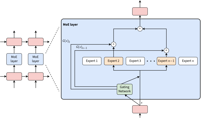
A Mixture of Experts (MoE) layer embedded within a recurrent language model. In this case, the sparse gating function selects two experts to perform computations. Their outputs are modulated by the outputs of the gating network. Adapted from: Outrageously Large Neural Networks: The Sparsely-Gated Mixture-of-Experts Layer
Noisy top-k gating. Instead of the softmax gating \(g(x) = \mathrm{Softmax}(x \cdot W_g)\), the router adds tunable Gaussian noise to its logits, which gives \(H(x)\), and sets the logits of all but the top-\(k\) experts to \(-\infty\) before the softmax, so that their gate values are 0:
\[G(x) = \mathrm{softmax}(\, \mathrm{KeepTopK}(\, H(x), k) \;)\] \[H(x)_i = (x \cdot W_g)_i + \mathrm{StandardNormal}() \cdot \mathrm{Softplus}((x \cdot W_{noise})_i)\]where \(\mathrm{Softplus}(x) = \log(1 + e^x)\) keeps the noise scale positive, and the noise helps balance the load (see the load loss below). The paper uses \(k > 1\): with \(k = 1\), the softmax of the single kept logit is always 1, so the router would receive no gradient (section 2.1 of the paper). Learning to route was thus thought to need at least two experts per token.
The shrinking batch problem. With a batch of \(T\) tokens, each expert receives on average only \(kT/N\) tokens. GPUs need large batches to amortize the cost of loading and updating the parameters, so a naive MoE becomes very inefficient as the number of experts grows. The paper grows the batch of each expert in two ways. With what is now called expert parallelism, the other layers and the router are data-parallel, but each expert has a single copy, on one device, which receives the relevant tokens of all devices. With convolutionality, the MoE processes all time steps of the previous layer together, as one big batch. For thousands of experts, a two-level hierarchical MoE reduces the branching factor: a primary router picks a sparse combination of secondary MoEs, each with its own router and on its own device.
Importance loss. To avoid overpowering (a few experts get most of the gate values) and starvation (some experts are never picked), an importance loss is added, equal to the square of the coefficient of variation of the importance values:
\[L_{importance} = w_{importance} \cdot CV(\, \mathrm{Importance}(X)\,)^2\]where \(CV = \sigma/\mu\) is the ratio of the standard deviation to the mean, \(\mathrm{Importance}(X)_i = \sum_{x \in X} G(x)_i\) is the sum of the gate values of expert \(i\) over a batch \(X\) (Eq. 6 in the paper), and \(w_{importance}\) is a hand-tuned scaling factor. In practice, the loss is zero when all experts have the same importance.
Load loss. Experts of the same importance may still receive different numbers of tokens (e.g. a few tokens with large gate values against many with small ones), which unbalances memory and compute across devices. A load loss balances the number of tokens instead. As this count is discrete and cannot be backpropagated, it uses a smooth estimate \(\mathrm{Load}(X)\):
\[L_{load} = w_{load} \cdot CV(\, \mathrm{Load}(X)\,)^2, \quad \text{with} \quad \mathrm{Load}(X)_i = \sum_{x \in X} P(x,i)\]where \(w_{load}\) is a hand-tuned scaling factor, and \(P(x,i) = Pr(H(x)_i \gt kth\_excluding(H(x), k, i))\) is the probability that \(G(x)_i\) is non-zero for a new random noise on element \(i\), keeping the noise of the other elements. Note that \(G(x)_i\) is non-zero if and only if \(H(x)_i\) is greater than the \(k\)-th greatest element of \(H(x)\), excluding \(H(x)_i\) itself (Appendix A of the paper).
For the same compute per token, the MoE models beat the LSTM baselines, and their perplexity kept improving with more experts, up to 65,536 experts in a hierarchical MoE. The authors claim “greater than 1000x improvements in model capacity with only minor losses in computational efficiency”. The experts also specialize in syntax and semantics (Appendix E, Table 9):
| Expert 381 | Expert 752 | Expert 2004 |
|---|---|---|
| … with researchers , … | … plays a core … | … with rapidly growing … |
| … to innovation . | … plays a critical … | … under static conditions … |
| … tics researchers . | … provides a legislative … | … to swift ly … |
| … the generation of … | … play a leading … | … to dras tically … |
| … technology innovations is … | … assume a leadership … | … the rapid and … |
| … technological innovations , … | … plays a central … | … the fast est … |
| … support innovation throughout … | … taken a leading … | … the Quick Method … |
| … role innovation will … | … established a reconciliation … | … rec urrent ) … |
| … research scienti st … | … played a vital … | … provides quick access … |
| … promoting innovation where … | … have a central … | … of volatile organic … |
| … | … | … |
Contexts corresponding to a few of the 2048 experts in the MoE layer in the encoder portion of the WMT’14 En→Fr translation model. For each expert \(i\), we sort the inputs in a training batch in decreasing order of \(G(x)_i\), and show the words surrounding the corresponding positions in the input sentences. Source: Outrageously Large Neural Networks: The Sparsely-Gated Mixture-of-Experts Layer
GShard: conditional computation for improved scaling
In 2020, GShard: Scaling Giant Models with Conditional Computation and Automatic Sharding scaled Transformer MoEs up to 600B parameters for machine translation, trained on 2048 TPU v3 accelerators in 4 days. Its main contribution is automatic sharding: the user annotates “a few critical tensors in the model with partitioning policies”, and an extension of the Accelerated Linear Algebra (XLA) compiler partitions the computation graph with a Single Program Multiple Data (SPMD) transformation. It generates a single program for all devices, which keeps the compilation time independent of the device count (Figure 2 in the paper).
The model replaces the feed-forward layer of every second Transformer block with a top-2 MoE layer, in the encoder and the decoder. The attention layers are data-parallel, while the experts, too large to be replicated, are sharded across devices. The encoder and its placement on several devices are illustrated below:
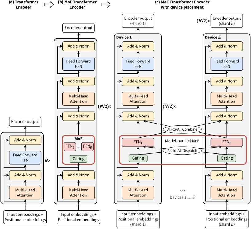
Illustration of scaling of Transformer Encoder with MoE Layers. The MoE layer replaces every other Transformer feed-forward layer. Decoder modification is similar. (a) The encoder of a standard Transformer model is a stack of self-attention and feed forward layers interleaved with residual connections and layer normalization. (b) Replacing every other feed-forward layer with an MoE layer gives the MoE Transformer Encoder. (c) When scaling to multiple devices, the MoE layer is sharded across devices, while all other layers are replicated. Adapted from: GShard: Scaling Giant Models with Conditional Computation and Automatic Sharding
In the picture, \(E\) is the number of experts, which is also the number of devices, and \(N\) is the number of layers; this post keeps \(N\) for the number of experts. Each device holds a shard of the input, a copy of the attention and dense feed-forward layers, and one expert of each MoE layer. In each MoE layer, an all-to-all dispatch sends each token to the devices of its experts, and an all-to-all combine sends the outputs of the experts back to the device of the token, where they are weighted by the gate values and summed.
Expert capacity. Each expert processes at most a fixed number of tokens per iteration, its expert capacity, of order \(O(T/N)\). GShard routes the tokens in groups of \(S\) tokens (each sequence in the implementation at the end of this post), and each expert takes at most \(2S/N\) tokens of a group (section 2.2 of the paper): the average \(S/N\), doubled because each token goes to up to two experts. The overflow tokens, whose experts are all full, skip the layer through the residual connection.
Random routing. The top expert always receives the token, but the second one only with probability \(2 g_2\), where the gate values \(g_1\) and \(g_2\) of the two experts are normalized to sum to 1 (Algorithm 1 in the paper). A second expert with a small gate value contributes little, so skipping it saves compute and overflow.
Auxiliary loss. The loss is \(L = l_{nll} + \alpha \cdot l_{aux}\), where \(l_{nll}\) is the negative log-likelihood, \(\alpha\) is a constant, and the auxiliary loss \(l_{aux}\) keeps a few experts from taking most tokens early in training:
\[l_{aux} = \frac{1}{N} \sum^N_{e=1} \frac{c_e}{S} \, m_e\]where \(c_e/S\) is the fraction of the \(S\) tokens of a group whose first choice is expert \(e\), and \(m_e\) is the mean gate value of expert \(e\) over the group. The loss approximates the mean square of \(c_e/S\), which is smallest when the tokens are spread evenly across the experts. \(m_e\) replaces one factor \(c_e/S\) because \(c_e/S\) comes from the selection of the experts, which is not differentiable.
Switch Transformers
MoEs were still held back by their complexity, communication costs and training instability. The 2021 paper Switch Transformers: Scaling to Trillion Parameter Models with Simple and Efficient Sparsity simplified the routing and delivered the first large MoEs trained in BF16. With Switch routing, each token goes to a single expert (top-1), whose output is multiplied by its router probability, a softmax over all experts, so the router still receives a gradient. Compared with the top-2 routing of GShard, this cuts the routing compute and the communication, and at least halves the expert capacity, while keeping the model quality, against the conjecture of the 2017 paper. The following picture illustrates a Switch Transformer encoder block:
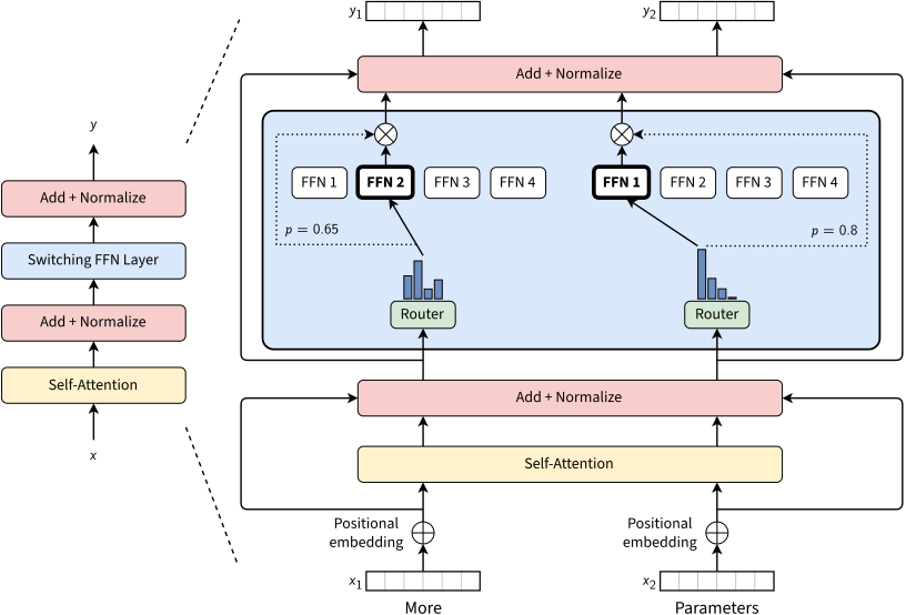
Illustration of a Switch Transformer encoder block. The dense feed forward network (FFN) layer of the Transformer is replaced by a sparse Switch FFN layer (light blue). The layer operates independently on the tokens in the sequence. Two tokens (x1 = “More” and x2 = “Parameters” below) are routed (solid lines) across four FFN experts; the router routes each token independently. The switch FFN layer returns the output of the selected FFN multiplied by the router gate value (dotted-line). Adapted from: Switch Transformers: Scaling to Trillion Parameter Models with Simple and Efficient Sparsity
Capacity factor. The expert capacity is the average number of tokens per expert, \(T/N\) for a batch of \(T\) tokens, times a capacity factor (Eq. 3 in the paper). As in GShard, the overflow tokens skip the layer through the residual connection. The routing of six tokens to three experts, one per device, with capacity factors of 1.0 and 1.5, is displayed below:
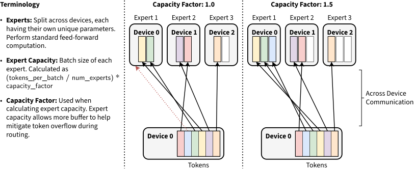
Illustration of token routing dynamics. Each expert processes a fixed batch-size of tokens modulated by the capacity factor. Each token is routed to the expert with the highest router probability, but each expert has a fixed batch size of (total_tokens / num_experts) × capacity_factor. If the tokens are unevenly dispatched then certain experts will overflow (denoted by dotted red lines), resulting in these tokens not being processed by this layer. A larger capacity factor alleviates this overflow issue, but also increases computation and communication costs (depicted by the empty white slots). Adapted from: Switch Transformers: Scaling to Trillion Parameter Models with Simple and Efficient Sparsity
With a capacity factor of 1.0, an expert that receives more tokens than the average drops the extra ones (the dotted red line), while another expert leaves a slot empty. With 1.5, no token is dropped, but more slots stay empty, so part of the compute and communication is spent on padding. Switch Transformers perform best at low capacity factors (1.0, 1.25), where they beat top-2 MoEs in quality and in time (Table 1 in the paper). Such low factors are the setting of large models, where memory is scarce.
Load balancing loss. A single auxiliary loss replaces the importance and load losses of the 2017 paper, and is added to the loss for every Switch layer. Given \(N\) experts and a batch of \(T\) tokens, \(f_i\) is the fraction of tokens dispatched to expert \(i\), and \(P_i\) is the mean router probability of expert \(i\) over the \(T\) tokens. The auxiliary loss is computed as (Eq. 4 to 6 in the paper):
\[loss = \alpha \cdot N \cdot \sum_{i=1}^{N} f_i \cdot P_i\]where \(\alpha\) is a hyper-parameter (\(10^{-2}\) in the paper). Ideally, all \(f_i\) and \(P_i\) are \(1/N\): the sum is then \(1/N\), so the factor \(N\) makes the loss equal to \(\alpha\) for any number of experts. It has the form of the auxiliary loss of GShard, with \(f_i\) in the role of \(c_e/S\) and \(P_i\) in the role of \(m_e\). Only \(P\) is differentiable, so the gradient lowers the router probabilities of the experts that receive the most tokens.
Distillation. The large sparse models can be distilled into small dense ones: “We reduce the model size by up to 99% while preserving 30% of the quality gains of the large sparse teacher”.
Expert-choice routing
All the schemes above are token-choice routing: each token picks its experts, so auxiliary losses and capacities are needed to balance the load. The 2022 paper Mixture-of-Experts with Expert Choice Routing reverses the choice: with expert-choice routing, each expert picks a fixed number of tokens, those with the highest router scores, so the load is balanced by construction. A token may then be processed by a variable number of experts, or by none. For the same compute, the paper reports a training convergence more than twice as fast as with the top-1 and top-2 gating of Switch Transformers and GShard.
Stable training with the router z-loss
Sparse models remained hard to train. The 2022 paper ST-MoE: Designing Stable and Transferable Sparse Expert Models introduces the router z-loss, which resolves the instabilities and slightly improves the model quality. Its ST-MoE-32B, a sparse model of 269B parameters with the compute of a dense 32B model, was the first sparse model to reach the state of the art in transfer learning.
Sparse models are sensitive to roundoff errors because the routers add exponential functions, which turn a small error of their input into a large error of their output (Section 3.4 of the paper). In BF16, large logits are rounded coarsely, which can change the router probabilities by a large amount. The z-loss is computed as:
\[L_z = \frac{1}{T} \sum_{i=1}^{T} \left( \log \sum_{j=1}^{N} e^{\ell_j^{(i)}} \right)^2\]where \(T\) is the number of tokens, \(N\) is the number of experts, and \(\ell^{(i)} = x^{(i)} \cdot W_g\) are the \(N\) router logits of the token \(x^{(i)}\) (Eq. 5 in the paper, which writes \(B\) for the number of tokens and \(x\) for the logits). It is added to the loss with a weight \(c_z = 0.001\). The term in the square is the LogSumExp of the logits, a smooth approximation of their maximum. So the z-loss is small only when the largest logit is close to 0, where BF16 is precise, as the gap between its representable numbers grows with their magnitude. Note that adding a constant to every logit leaves the softmax unchanged, but not the z-loss.
Mixtral 8x7B: total and active parameters
At the time of writing, the state-of-the-art MoE was Mixtral 8x7B, presented in the 2024 paper Mixtral of Experts. It has the architecture of Mistral 7B (Table 1 in the paper), except that it supports a fully dense context of 32k tokens, and each feed-forward block is replaced by 8 experts. It routes each token to 2 experts, so “each token has access to 47B parameters, but only uses 13B active parameters during inference”.
Compared with GShard, the MoE is in every layer instead of every second one, and the second expert is not picked at random. The gating is \(G(x) = \mathrm{Softmax}(\mathrm{TopK}(x \cdot W_g))\), where \(\mathrm{TopK}(\ell)_i = -\infty\) if the logit \(\ell_i\) is not among the top-\(k\), i.e. the noisy top-\(k\) gating of 2017 without the noise. With SwiGLU experts, the output for an input \(x\) is computed as:
\[y = \sum_{i=1}^{N} \mathrm{Softmax}(\mathrm{Top2}(x \cdot W_g))_i\cdot \mathrm{SwiGLU}_i(x),\]where \(N = 8\) is the number of experts and \(\mathrm{SwiGLU}_i\) is expert \(i\).
The name 8x7B suggests 56B parameters, but only the feed-forward blocks are replicated, while the attention layers, the routers, the normalization layers and the embeddings are shared. The 47B total (or sparse) parameters grow with the number of experts and set the memory of the model, while the 13B active parameters grow with \(k\) and set its compute per token. For expert parallelism (EP), the paper notes that “EP introduces challenges in load balancing, as it is essential to distribute the workload evenly across the GPUs to prevent overloading individual GPUs or hitting computational bottlenecks”. The next section implements expert parallelism in PyTorch.
Distributed implementation in PyTorch
The MoE workflow is a four-step algorithm, best illustrated in the MegaBlocks paper:
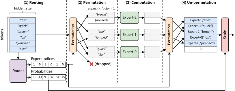
A Mixture-of-Experts Layer. Shown for num_experts=3, top_k=1 and capacity_factor=1 with the prevalent, token dropping formulation. First (1), tokens are mapped to experts by the router. Along with expert assignments, the router produces probabilities that reflect the confidence of the assignments. Second (2), the feature vectors are permuted to group tokens by expert assignment. If the number of tokens assigned to an expert exceeds its capacity, extra tokens are dropped. Third (3), the expert layers are computed for the set of tokens they were assigned as well as any padding needed for unused capacity. Lastly (4), the results of the expert computation are un-permuted and weighted by the router probabilities. The outputs for dropped tokens are shown here set to zero. Adapted from: MegaBlocks: Efficient Sparse Training with Mixture-of-Experts
The tokens travel to the experts and back with all-to-all collectives, and their gradients must make the same trip in reverse during the backward pass. dist.all_to_all_single has no backward pass, so it is wrapped in an autograd function whose backward pass runs the opposite all-to-all:
class AllToAll(torch.autograd.Function):
  """ all_to_all_single along the first dimension, whose backward pass sends the gradients back """

  @staticmethod
  def forward(ctx, x, output_split_sizes, input_split_sizes):
    ctx.split_sizes = output_split_sizes, input_split_sizes
    out = x.new_empty(sum(output_split_sizes), *x.shape[1:])
    dist.all_to_all_single(out, x.contiguous(), output_split_sizes, input_split_sizes)
    return out

  @staticmethod
  def backward(ctx, grad_out):
    output_split_sizes, input_split_sizes = ctx.split_sizes
    grad_x = grad_out.new_empty(sum(input_split_sizes), *grad_out.shape[1:])
    dist.all_to_all_single(grad_x, grad_out.contiguous(), input_split_sizes, output_split_sizes)
    return grad_x, None, None
The distributed MoE block is then defined as MoE_dist, with a replicated (data-parallel) router and a local expert. For the sake of simplicity, there is a single expert per GPU and no load balancing loss, and the tokens that exceed each expert’s capacity are dropped:
class MoE_dist(nn.Module):
  def __init__(self, n_embd, k=2, capacity_factor=1.25, padding_val=0, local_rank=None):
    super().__init__()
    self.capacity_factor = capacity_factor
    self.padding_val = padding_val
    self.num_experts = dist.get_world_size() # 1 expert per GPU
    self.k = k

    if local_rank is None:
      local_rank = int(os.environ.get("LOCAL_RANK", dist.get_rank()))
    device = torch.device("cuda", local_rank)

    self.router = DDP(Router(n_embd, self.num_experts).to(device), device_ids=[local_rank])
    self.expert = FeedForward(n_embd).to(device)
Here, the Router is a feed-forward network that takes the embedding of a token as input and outputs a distribution of allocations (probabilities) over the experts. Also, the code assumes there is only one expert per process, so the process id matches the expert id, and the number of experts matches the number of processes.
The routing step computes the top-k expert assignments of each token, i.e. the expert ids in topk_experts and the corresponding probabilities in topk_probs, and groups them by expert:
  def forward(self, x):
    # x: B*S*E
    B, S, E = x.shape
    global_rank = dist.get_rank()
    probs = self.router(x) # get assignments from router, shape B*S*n_experts
    topk_probs, topk_experts = torch.topk(probs, k=self.k, dim=-1) # B*S*k

    ids_per_expert = [ (topk_experts==expert).nonzero() for expert in range(self.num_experts) ]
    probs_per_expert = [ topk_probs[topk_experts==expert] for expert in range(self.num_experts) ]
The following permutation step, the all-to-all dispatch of the GShard picture, selectively sends the tokens to each expert’s processor. It uses collective communication, in two steps. First, an all_to_all operation exchanges the number of items to send/receive, needed to allocate the receive buffers. Then, based on those counts, an all_to_all_single call exchanges the metadata of the tokens, and an AllToAll call exchanges the tokens themselves:
    device = x.device

    # all-to-all to exchange the count of inputs to send/receive to/from each processor
    send_count = [torch.tensor([len(ids)], dtype=torch.int64, device=device) for ids in ids_per_expert]
    recv_count = [torch.tensor([0], dtype=torch.int64, device=device) for _ in ids_per_expert]
    dist.all_to_all(recv_count, send_count)
    fn_count = lambda tensor, scale=1: [x.item()*scale for x in tensor]

    # send/receive the metadata (b, s, which_topk) to/from the appropriate processors
    M = ids_per_expert[0].shape[-1] # number of columns in metadata
    send_ids = torch.cat(ids_per_expert, dim=0).to(device)
    send_ids[:,0] += global_rank*B # add processor's batch offset
    recv_ids = torch.zeros(sum(recv_count)*M, dtype=send_ids.dtype, device=device)
    dist.all_to_all_single(recv_ids, send_ids.flatten(), fn_count(recv_count,M), fn_count(send_count,M))
    recv_ids = recv_ids.view(-1, M) # reshape to M columns

    # send/receive input tokens to/from the appropriate processors
    send_toks = torch.cat([ x[ids[:,0], ids[:,1]] for ids in ids_per_expert], dim=0).to(device)
    recv_toks = AllToAll.apply(send_toks, fn_count(recv_count), fn_count(send_count)) # sum(recv_count) rows, E columns
The all-to-all collective is illustrated in the following diagram:
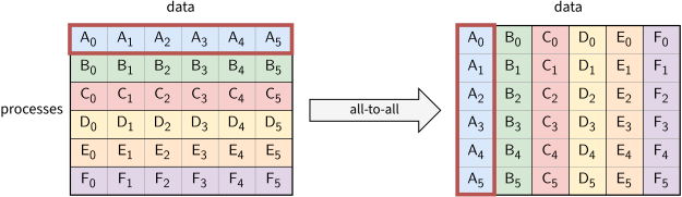
An illustration of the MPI all-to-all collective operation. When each process sends one element to each process, the operation is equivalent to a distributed matrix transpose: the row framed in red before the all-to-all (left), the data of process A, becomes the first column after the all-to-all (right). A single-element all-to-all exchanges the number of items to be sent and received among processes. These counts are then used by two all-to-alls with variable-sized elements in the permutation step, one for the token metadata and one for the tokens. In the un-permutation step, another all-to-all performs the reverse communication by swapping the send and receive counts and buffers. Adapted from: MPI Tutorial, Shao-Ching Huang, IDRE High Performance Computing Workshop, 2013
The computation step reshuffles the received data into a 3D batch of size Rows x Capacity x Embedding, cropping or padding each sequence to the capacity of the expert:
    # group received metadata by row id
    uniq_rows, recv_row_lens = recv_ids[:,0].unique(sorted=True, return_counts=True)
    recv_row_offsets = [0] + torch.cumsum(recv_row_lens, dim=0).tolist()
    recv_row_slice = lambda row: slice(recv_row_offsets[row], recv_row_offsets[row+1])

    # crop or pad received items PER SENTENCE to max capacity. Batch shape: Rows * Capacity * E
    capacity = int(S / self.num_experts * self.capacity_factor)
    pad_fn = lambda toks, value = self.padding_val: F.pad(toks, (0,0,0,capacity-toks.shape[0]), value=value) # pad or crop
    batch_row_len = torch.tensor([ min(recv_row_lens[r], capacity) for r in range(len(uniq_rows))], device=device)

    if len(uniq_rows) > 0: # the expert may receive no tokens
      batch_toks = torch.stack([ pad_fn(recv_toks[recv_row_slice(i)][:capacity]) for i in range(len(uniq_rows))], dim=0).to(device)
      batch_toks = self.expert(batch_toks) # Rows * Capacity * E
The output of the expert is stored in batch_toks. The following un-permutation step, the all-to-all combine of the GShard picture, performs an AllToAll with the opposite communication of the permutation step. This populates the all-to-all output buffer with the partial results of all experts.
    # scatter computed outputs back into recv_toks (only for the non-padding part). out_flat is computed from recv_toks
    # so that every process runs both all-to-alls of the backward pass, even if its expert received no tokens
    out_flat = recv_toks * 0 + self.padding_val
    cursor = 0
    for r in range(len(uniq_rows)):
      n = int(batch_row_len[r].item())
      out_flat[cursor:cursor+n] = batch_toks[r, :n]
      cursor += int(recv_row_lens[r].item())

    # send back
    x = AllToAll.apply(out_flat, fn_count(send_count), fn_count(recv_count)) # sum(send_count) rows, E columns
Finally, the un-permutation step also scales the outputs: it computes, for each token, the sum of the outputs of its top-k experts, weighted by the router probabilities. The outputs arrive grouped by expert, so each one is added at the position of its token, given by the metadata (b, s) sent in the permutation step:
    x = x * torch.cat(probs_per_expert).view(-1,1) # multiply by router probabilities
    rows = (send_ids[:,0] - global_rank*B) * S + send_ids[:,1] # position b*S+s of each output, without the batch offset
    out = torch.zeros(B*S, E, dtype=x.dtype, device=device).index_add(0, rows, x) # sum the top-k outputs of each token
    return out.view(B,S,E)
Applying the MoE to an existing LLM
Remember that the MoE module can replace the feed-forward module in existing architectures. So here it is applied to the GPT2-based GPTlite model built in a previous post. This is straightforward: all that is needed is to distribute its modules in a Distributed Data Parallel fashion, except the feed-forward module of the transformer block, which is replaced with the expert-parallel MoE:
  # ddp function takes a torch module and distributes it in a data parallel fashion
  ddp = lambda module: DDP(module.to(device), device_ids=[local_rank])

  model = GPTlite(vocab_size) # instantiate GPTlite locally
  model.token_embedding_table = ddp(model.token_embedding_table)
  model.position_embedding_table = ddp(model.position_embedding_table)
  model.ln = ddp(model.ln)
  model.lm_head = ddp(model.lm_head)
  for b, block in enumerate(model.blocks):
    block.sa = ddp(block.sa)
    block.ln1 = ddp(block.ln1)
    block.ln2 = ddp(block.ln2)
    block.ffwd = MoE_dist(n_embd=n_embd) # replace FeedForward with a MoE (parallelism handled inside)
The rest of the training and optimization algorithm needs no changes.
For further reading, LatentMoE, used in Nemotron 3, runs the experts on a smaller projection of each token, which cuts their weights and the all-to-all traffic, and spends the savings on more experts, with more of them per token.