Distributed training: pipeline parallelism (1F1B, Zero Bubble, Dual Pipe)
In this post we will discuss and implement pipeline parallelism. Pipeline parallelism is just another possible dimension of model parallelism on the universe of data, tensor, pipeline, tensor, context, sequence and expert parallelism.
Imagine we have a model that is too large to fit in the local memory of a single process. A simple way to overcome this is to split the model across the layer dimension and delegate a subset of layers to each process. Then we can do a forward and backward pass by communicating activations and gradients between connecting processes. Each process is responsible for a subset of layers and is called a stage. This type of parallelism is called pipeline parallelism. The following picture gives us a simple illustration of the process:
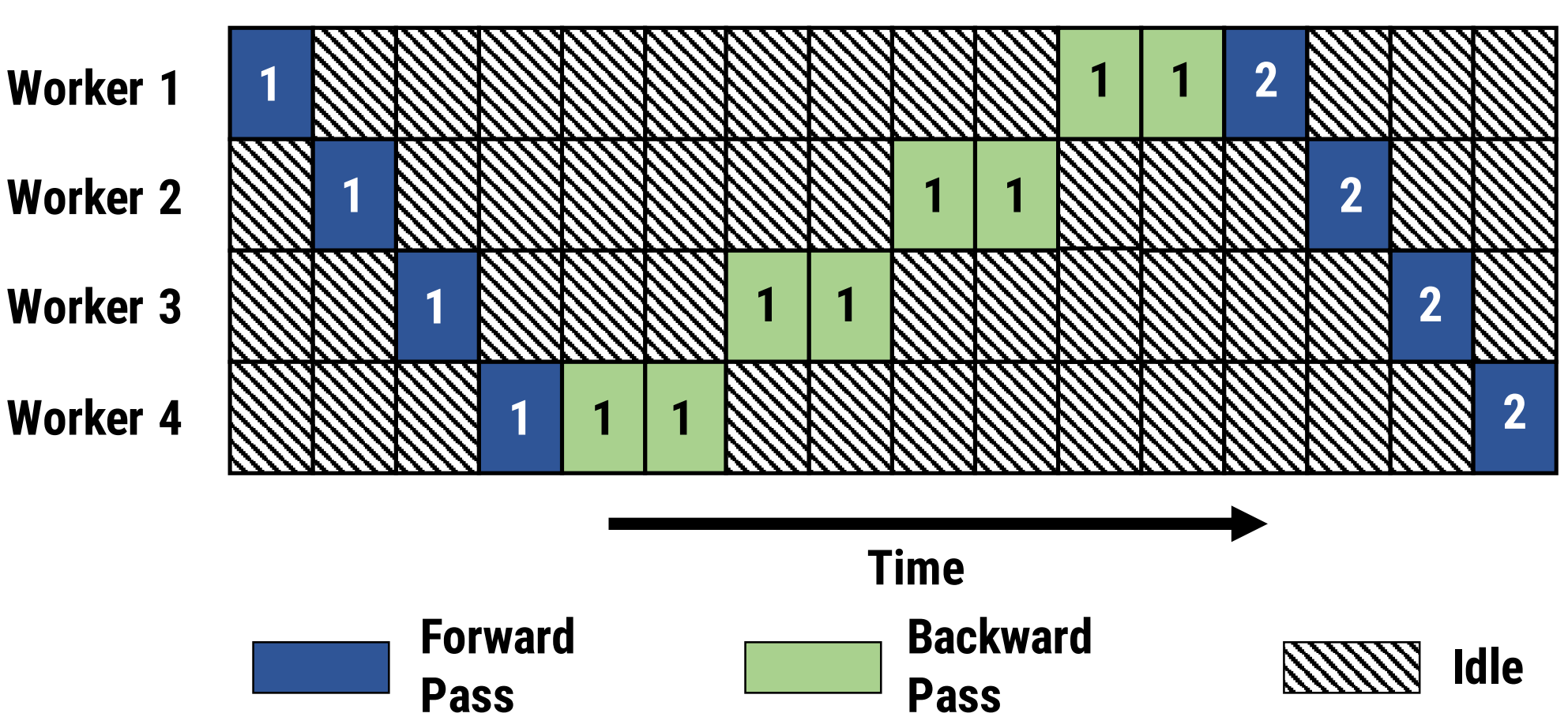
Left-to-right timeline of a serial execution of the training of a model divided across 4 compute units (Workers) and 4 stages. Blue squares represent forward passes. Green squares represent backward passes and last for twice the amount of the forward pass. The number on each square is the data sample index. Black squares represent moments of idleness, i.e. of a worker not performing any computation. Source: PipeDream: Generalized Pipeline Parallelism for DNN Training (Microsoft, arXiv)
Now note that the above method would yield a low utilization of compute resources: processes would always have to wait for connecting layers in different processes to be computed before being able to do their share of the forward/backward compute. So pipeline parallelism is usually combined with micro-batching / gradient accumulation. In practice, we can split the mini-batch in several micro-batches and pass them sequentially to the first process of the pipeline. When a process finishes the current micro-batch, it sends its activations to the following process and receives the next micro-batch activations from the previous process. This is mathematically equivalent to regular gradient accumulation. This approach is detailed in the paper GPipe: Efficient Training of Giant Neural Networks using Pipeline Parallelism (Google, 2018, arXiv) and can be illustrated as:
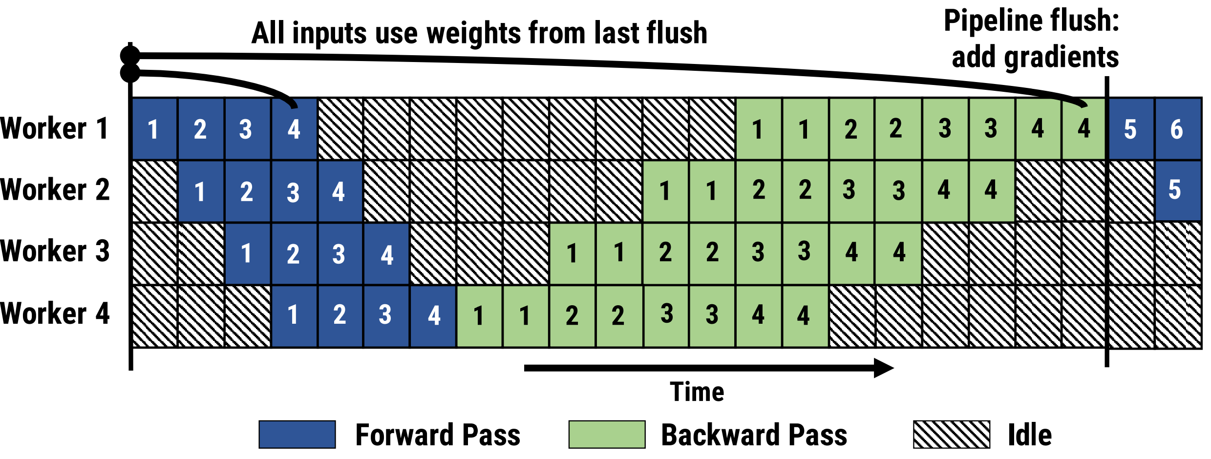
A pipeline execution with gradient accumulation, computed as a sequence of 4 micro-batches. Source: PipeDream: Generalized Pipeline Parallelism for DNN Training (Microsoft, arXiv)
Setting a high micro-batching factor can lead to high memory usage, as we have to store activations until we finish the backward pass for the current mini-batch. This can be improved by (1) activation offloading, which stores and loads activations to/from the CPU when needed; and (2) activation checkpointing at the beginning of every stage, which recomputes activations during the backward pass when needed instead of keeping them always in memory.
The other hyper-parameter we have to define is the number of stages. Up until now, the examples above used a number of stages equivalent to the number of workers, i.e. a single pipeline that spans all workers. However, we can have multiple pipelines in parallel and combine pipeline parallelism with other dimensions of parallelism. As an example, if you’d combine pipeline and data parallelism on an 8-GPU network:
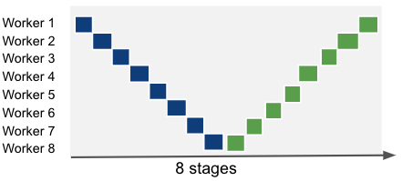
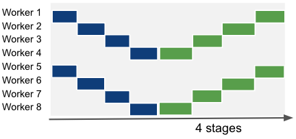
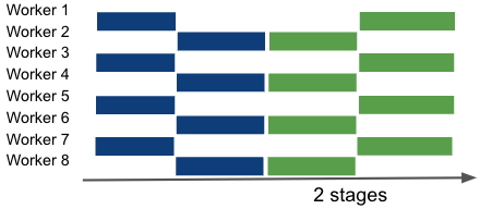
An illustration of different combinations of pipeline and data parallelism. Left: 8 pipeline-parallel workers. Center: 2 data-parallel groups of 4 pipeline-parallel workers. Right: 4 data-parallel groups of 2 pipeline-parallel workers.
You will notice that no matter the pipeline configuration we use, there are periods of idleness that we cannot remove. With this in mind, there is plenty of work ongoing to improve this. As an example, PipeDream: Generalized Pipeline Parallelism for DNN Training (Microsoft, arXiv) is a pipeline method that overlaps forward and backward passes of different mini-batches, by keeping track of the version (micro-batch id) and storing several versions of activations and parameters whose backward pass hasn’t completed:
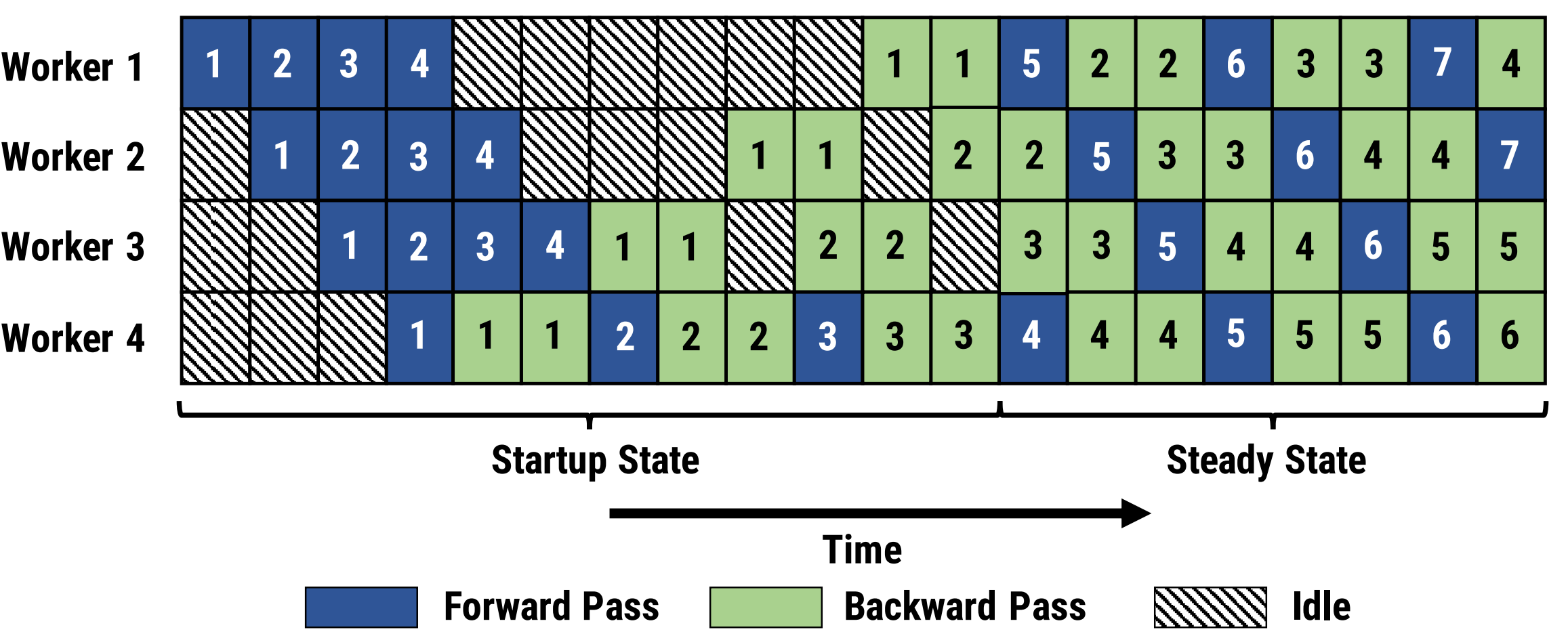
The PipeDream scheduling algorithm. Several forward passes can be in flight, even if they derive from different micro-batches. Backward passes are prioritized over forward passes on each worker. Source: PipeDream: Generalized Pipeline Parallelism for DNN Training (Microsoft, arXiv)
Where’s the caveat? In practice, mixing forward and backward passes from different mini-batches can lead to wrong parameter updates. Therefore, the authors perform versioning of the parameters, effectively having several versions of the same parameters in the model. Forward passes use the latest version of the model layers, and the backward may use a previous version of activations and optimizer state to compute the gradients. This leads to a substantial increase in memory requirements.
Implementing pipeline parallelism with PyTorch
Before we jump into DeepSpeed’s 1F1B pipeline engine, it is helpful to implement the simplest possible pipeline parallel training loop in plain PyTorch. The goal of this section is not performance. It is simply to show the mechanics of:
- partitioning a model into
num_stagessequential stages, - sending activations forward stage-by-stage,
- sending activation gradients backward stage-by-stage,
- and performing one optimizer step per mini-batch (optionally using micro-batches).
To match the scheduling shown in the figure (no overlapping micro-batches between stages), we use a non-overlapped schedule: we run an entire micro-batch through all forward stages, then run its backward pass all the way back, and only then move to the next micro-batch. This is conceptually the most straightforward schedule, but it leaves lots of bubbles (idle time) and is mainly for learning/debugging.
Below is a minimal example. It assumes:
- one pipeline group of size
num_stages(oftennum_stages == world_sizefor a single pipeline), - each rank is one stage (
stage_id = rank_in_pipeline), - each stage holds a
nn.Sequentialblock of layers.
Note: This is a toy implementation. In real systems you also need: shape/metadata communication, mixed precision, activation checkpointing, pipeline/data parallel composition, and better schedules (like 1F1B).
import torch
import torch.distributed as dist
import torch.nn as nn

def split_layers(layers, num_stages):
    # naive equal split (by count). Real code should load-balance by params/runtime.
    idx = torch.arange(len(layers))
    chunks = torch.chunk(idx, num_stages)
    return [nn.Sequential(*[layers[i] for i in c.tolist()]) for c in chunks]

def pipeline_step_no_overlap(x_mb, y_mb, stage, stage_id, num_stages, criterion):
    """Run one micro-batch through the full pipeline forward, then full backward."""

    # ---- Forward ----
    if stage_id == 0:
        act = x_mb.detach().requires_grad_(True)
        act = stage(act)
        dist.send(act, dst=stage_id + 1)
    elif stage_id < num_stages - 1:
        # receive activation from previous stage
        act = torch.empty_like(x_mb)  # placeholder; in practice you must know the correct shape
        dist.recv(act, src=stage_id - 1)
        act = act.detach().requires_grad_(True)
        act = stage(act)
        dist.send(act, dst=stage_id + 1)
    else:
        # last stage: receive, compute loss
        act = torch.empty_like(x_mb)  # placeholder; in practice you must know the correct shape
        dist.recv(act, src=stage_id - 1)
        act = act.detach().requires_grad_(True)
        out = stage(act)
        loss = criterion(out, y_mb)
        loss.backward()
        # send grad of activation to previous stage
        dist.send(act.grad, dst=stage_id - 1)
        return loss.detach()

    # ---- Backward (non-last stages) ----
    # receive grad from next stage, backprop through local stage, send to previous
    grad_act = torch.empty_like(act)
    dist.recv(grad_act, src=stage_id + 1)

    act.backward(grad_act)

    if stage_id > 0:
        dist.send(act.grad, dst=stage_id - 1)

    return None

def train_one_minibatch(model_layers, num_stages, optimizer, criterion, x, y, micro_batches=1):
    """Each rank runs only its local stage."""
    rank = dist.get_rank()
    stage_id = rank  # single pipeline group example

    stages = split_layers(model_layers, num_stages)
    stage = stages[stage_id].to(x.device)

    optimizer.zero_grad(set_to_none=True)

    x_mbs = x.chunk(micro_batches, dim=0)
    y_mbs = y.chunk(micro_batches, dim=0)

    loss_out = None
    for x_mb, y_mb in zip(x_mbs, y_mbs):
        loss = pipeline_step_no_overlap(x_mb, y_mb, stage, stage_id, num_stages, criterion)
        if loss is not None:
            loss_out = loss_out + loss if loss_out is not None else loss

    # Each stage has its own optimizer step (weights are disjoint across stages)
    optimizer.step()

    return loss_out
This shows the core idea: activations flow forward, gradients flow backward. The remaining sections use DeepSpeed to do the same thing, but efficiently and with better schedules (1F1B), load-balancing, activation checkpointing, and integration with other forms of parallelism.
Implementing pipeline parallelism with DeepSpeed
The pipeline parallelism algorithm implemented in DeepSpeed is the PipeDream-Flush implementation with default 1F1B scheduling (1 forward pass followed by 1 backward pass), however it is possible to extend pipeline parallelism to other algorithms. The 1F1B algorithm performs a sequence of forward passes, and asynchronously starts the backward pass for each micro-batch forward pass completed. It then waits for all forward and backward passes to complete before starting the new mini-batch.
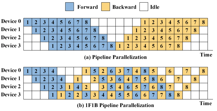
Regular and 1F1B pipeline algorithms diagram. Source: Training and Serving System of Foundation Models: A Comprehensive Survey
We will add pipeline parallelism to the GPTlite model implemented in the previous post, and enable it by passing the number of stages as the ---pipeline_num_stages argument (default: 0, no pipelining) on the command line:
## train.py

def get_cmd_line_args(description='GPT lite on DeepSpeed'):
  # ...
  parser.add_argument('--pipeline-parallel-size', type=int, default=0,
                      help='enable pipeline parallelism with N stages (0 means disabled)')
  # ...
DeepSpeed supports pipeline parallelism on any sequence of network blocks in a nn.Sequential container or list, that will be broken into pipeline stages. We’ll expose pipeline parallelism in our model by creating a method to_layers() in GPTlite, that returns the sequence of actions to be executed. Note that to_layers() follows the same order as the forward pass of GPTlite, and that self.blocks is of type nn.Sequential:
## gptlite.py

class GPTlite(nn.Module):
  # ...
  def to_layers(self):
      layers = [
          lambda idx:
            self.token_embedding_table(idx) +
            self.position_embedding_table(torch.arange(idx.shape[1]).to(idx.device)),
          *self.blocks,
          self.ln,
          self.lm_head,
      ]
      return layers
Note that the output of layers is of shape B,T,C which is incompatible with CrossEntropyLoss in PyTorch. A quick fix is to simply add lambda logits: torch.swapaxes(logits, 1, 2) to to_layers() to make it of shape B,C,T. However when you try to back-propagate, you may bump into the error RuntimeError: element 0 of tensors does not require grad and does not have a grad_fn, as discussed in bugs 4279 and 4479, and you’d have to use outputs = outputs.requires_grad_(True) to fix it. Alternatively, you can adapt the loss function to do the view/reshape change instead. It is a cleaner approach, and will be useful later for the pipeline parallelism use case:
## train.py

class CrossEntropyLoss_FlatView(torch.nn.Module):
  def forward(self, logits, labels):
    B, T, C = logits.shape
    logits = logits.view(B*T, C)
    labels = labels.view(-1)
    return torch.nn.functional.cross_entropy(logits, labels)

def main_deepspeed(n_epochs=100, random_seed=42):
  # ...
  criterion = CrossEntropyLoss_FlatView()  # initialize loss function
As a next step, in our DeepSpeed initialization code, we must create a pipeline wrapper around our model. This wrapped model is the new model variable that will be passed to deepspeed.initialize():
## gptlite.py

def get_model(criterion, vocab_size, pipeline_num_stages=0):
  # ...
  if pipeline_num_stages:
    deepspeed.runtime.utils.set_random_seed(random_seed)
    pipe_kwargs={
      'num_stages': pipeline_num_stages,
      'loss_fn': criterion,
      }
    model = gptlite.GPTlite(vocab_size).to(device_str)
    model = deepspeed.pipe.PipelineModule(layers=model.to_layers(), **pipe_kwargs)
  else:
    # ... as before: model = gptlite.GPTlite(vocab_size)
Finally, the training iteration code in the pipelining use case is reduced to a call to engine.train_batch(), that is equivalent to a forward pass, backward pass and gradient updates of an entire mini-batch of size engine.gradient_accumulation_steps() micro-batches:
## train.py

def main_deepspeed(n_epochs=100, random_seed=42):
  # ...
  for epoch in range(n_epochs):
    if pipeline_num_stages:
      step_count = len(train_dataset) // engine.gradient_accumulation_steps()
      for step in range(step_count):
        loss = engine.train_batch()
    else:
      # ... forward, backward, and update step as before
An important nuance: by default, pipeline parallelism expects all mini-batches of the dataset (i.e. in every call to train_batch()) to be of the same shape. If this is not the case, you can reset the shapes at the onset of every mini-batch by running engine.reset_activation_shape(), and this will introduce an additional communication step to broadcast the shapes of the first micro-batch as the default for the remaining micro-batches. However, it is not possible to have different shapes across micro-batches, and the only workaround is to trim or pad all micro-batches of a mini-batch to the same shape beforehand.
As a final remark, pipeline parallelism is not compatible with ZeRO stages 2 or 3, as discussed here.
Increasing compute and memory efficiency with LayerSpec (optional)
The implementation of pipelining for the GPTlite model above is neither memory efficient nor scalable as each GPU replicates the whole model in memory. See Memory-Efficient Model Construction for details. So we will use the DeepSpeed class LayerSpec (API) that delays the construction of modules until the model layers have been partitioned across workers, therefore having each worker allocate only the layers it’s assigned to. To do this, we will create a new model class GPTlitePipeSpec that inherits from PipelineModule with an __init__ method that follows very closely the forward() pass in the original GPTlite.
The tricky bit here is that the LayerSpec constructor only works with the type nn.Module as argument, and some operations, specifically the sum of embeddings in forward(), is not of type nn.Module. To overcome this, we create the class EmbeddingsSum that encapsulates that logic into an nn.Module. We will also use CrossEntropyLoss_FlatView as the loss function. The full implementation for the pipeline class is then:
## gptlite.py

from deepspeed.pipe import PipelineModule, LayerSpec

class GPTlitePipeSpec(PipelineModule):

  class EmbeddingsSum(nn.Module):
    """Converts tok_emb + pos_emb into an nn.Module. Required for LayerSpec."""

    def __init__(self, vocab_size):
      super().__init__()
      self.token_embedding_table = nn.Embedding(vocab_size, n_embd)
      self.position_embedding_table = nn.Embedding(block_size, n_embd)

    def forward(self, idx):
      B, T = idx.shape
      tok_emb = self.token_embedding_table(idx)
      pos_emb = self.position_embedding_table(torch.arange(T).to(idx.device))
      return tok_emb + pos_emb

  def __init__(self, vocab_size, pipe_kwargs):
    self.specs = \
      [ LayerSpec(GPTlitePipeSpec.EmbeddingsSum, vocab_size) ] + \
      [ LayerSpec(Block, n_embd, n_head) for _ in range(n_layer)] + \
      [ LayerSpec(nn.LayerNorm, n_embd),
        LayerSpec(nn.Linear, n_embd, vocab_size, bias=False) ]
    super().__init__(layers=self.specs, **pipe_kwargs)
then we add the flag --pipeline_spec_layers to the command line arguments, so that we can optionally enable this feature:
## train.py

def get_cmd_line_args():
  # ...
  parser.add_argument("--pipeline_spec_layers", action="store_true",
                      help="enable LayerSpecs in pipeline parallelism")
and change the get_model() method to retrieve the efficient pipeline variant as:
## gptlite.py

def get_model(criterion, vocab_size, pipeline_num_stages=0, pipeline_spec_layers=False):

  if pipeline_num_stages:
    if pipeline_spec_layers:
      model = GPTlitePipeSpec(vocab_size, pipe_kwargs=pipe_kwargs)
    else:
      # ... GPTlite model as before
We will denominate the LayerSpec-based implementation of pipeline parallelism by memory-efficient pipelining.
For heterogeneous models, load balancing of the model across GPUs may be an issue. There are several metrics to load balance from: runtime, memory usage, parameter count, etc. Here, we will not tune the load balancing method for pipeline modules, and will instead use the default partition_method=parameters. This assigns layers to stages in a way that load-balances parameters, i.e. stages may have different lengths. Finally, in the extreme case the 1F1B algorithm is not the pipeline algorithm we want, we can extend pipeline parallelism with a different algorithm.
Activation checkpointing
Introducing activation checkpointing at every X layers in our pipeline is straightforward, we just need to specify that interval in the argument activation_checkpoint_interval in the PipelineModule constructor:
#gptlite.py

def get_model(criterion, vocab_size, pipeline_num_stages=0, \
  pipeline_spec_layers=False, activation_checkpoint_interval=0):

  if pipeline_num_stages:
    pipe_kwargs={ # ...
      'activation_checkpoint_interval': args.activation_checkpoint_interval,
    }
  # ....
However, activation checkpointing is also tricky to configure when using pipelining if the checkpoint layer falls in another GPU. The rationale is that if a checkpoint layer falls in a different GPU than the layer being back-propagated, this requires extra communication. This is a use case that I believe DeepSpeed is not handling correctly, so make sure there’s a checkpoint layer at the beginning of the first block on each GPU.
Gradient accumulation and micro-batching
We can define the micro-batching level by setting the fields train_micro_batch_size_per_gpu (defaulted to train_batch_size) or gradient_accumulation_steps (defaulted to 1) in the DeepSpeed config file. At runtime, the number of micro-batches can be retrieved by engine.gradient_accumulation_steps().
Results
We changed our config to ds_config.json to run ZeRO stage 1 and tested our execution with different stage count and the memory-efficient SpecLayer implementation of our GPT model (with --pipeline_num_stages <num_stages> --pipeline_spec_layers). We did not use activation checkpointing due to an open bug 4279. We tested 1, 2, 4 and 8 pipeline stages per run. We rely on the default DeepSpeed algorithm for load balancing of stages, based on the parameter count. As an example, for the partitioning of GPTlite pipeline across 8 GPUs and 4 stages, it outputs:
RANK=0 STAGE=0 LAYERS=4 [0, 4)   STAGE_PARAMS=21256704 (21.257M)
RANK=2 STAGE=1 LAYERS=3 [4, 7)   STAGE_PARAMS=21256704 (21.257M)
RANK=4 STAGE=2 LAYERS=3 [7, 10)  STAGE_PARAMS=21256704 (21.257M)
RANK=6 STAGE=3 LAYERS=6 [10, 16) STAGE_PARAMS=21308160 (21.308M)
Pipelining with optimized vs non-optimized memory efficiency implementation. Using the SpecLayer-based implementation of the PipelineModule in our pipeline runs resulted in a reduction of about 40% in memory consumption for the GPTlite and deep benchmark models when running pipeline parallelism with the highest stage count (8).
Memory usage: on pipeline parallelism, I noticed that the first GPU seems to require a higher amount of memory when compared to the remaining GPUs. This should not be the case, particularly on the deep benchmark model where we can guarantee a quasi-ideal stage partitioning across GPUs. This disparity in memory usage on GPU 0 is the main indicator of the maximum memory required, and balancing this would bring that value down. I opened a bug report with DeepSpeed and will wait for their feedback or fix to correct this analysis.
This code is available in the GPTlite-distributed repo, if you feel like giving it a try. I will try to add detailed results for pipeline parallelism in the future when time allows.
Beyond 1F1B: reducing the pipeline bubble
Even with 1F1B, every stage idles for (p-1)(F+B) per iteration, where p is the number of stages and F and B are the times of the forward and backward pass of one micro-batch on one stage. Relative to the compute of m micro-batches, this is a bubble fraction of (p-1)/m, so 1F1B can only reduce it with more micro-batches per iteration (i.e. a larger batch or smaller micro-batches) or with fewer stages. Newer schedules attack the bubble directly. They are not part of DeepSpeed, where they would require a custom schedule, but they are available in Megatron-LM, in PyTorch’s torch.distributed.pipelining and in DeepSeek’s DualPipe repository.
The diagrams in this section were generated from the reference implementation of each schedule, for 4 GPUs and 8 micro-batches. Time is normalized so that every GPU performs the same amount of compute in all diagrams: a forward pass takes 1 unit and a backward pass takes 2 units (1+1 when it is split into the gradients for inputs and for weights, as explained below), and schedules that place two model chunks on each GPU run each chunk in half the time. Communication time is not modeled. The number in each cell is the micro-batch id, gray cells are idle time, and the dashed line marks the end of the 1F1B schedule.
Interleaved 1F1B
Efficient Large-Scale Language Model Training on GPU Clusters Using Megatron-LM (NVIDIA, 2021, arXiv) assigns several non-contiguous chunks of layers (virtual stages) to each GPU, instead of a single block of consecutive layers. With 4 GPUs and 2 chunks per GPU, the model is split into 8 chunks, GPU 0 holds chunks 0 and 4, GPU 1 holds chunks 1 and 5, and so on, so every micro-batch loops through the GPUs twice. Smaller chunks make the pipeline fill and drain faster, and the bubble shrinks by the number of chunks per GPU v, to (p-1)(F+B)/v. The price is v times more point-to-point communication, and more activation memory, as the first GPU keeps more micro-batches in flight. The original implementation also requires the number of micro-batches to be a multiple of the number of GPUs. This schedule is available in Megatron-LM and as ScheduleInterleaved1F1B in PyTorch.
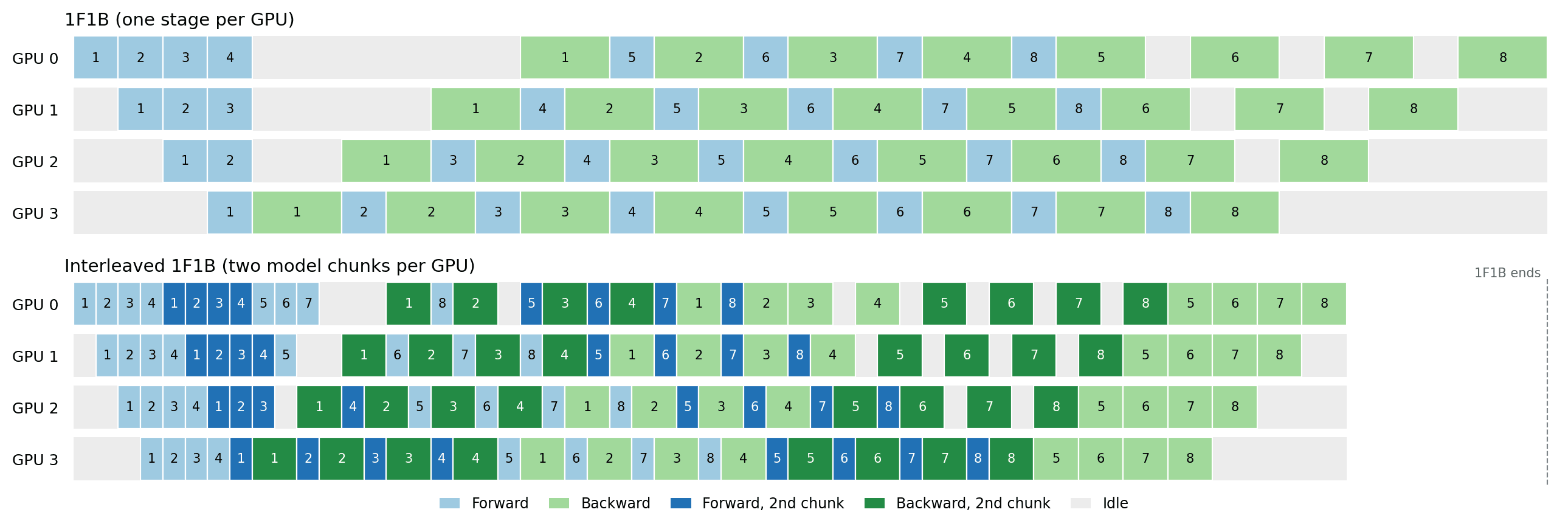
1F1B (top) and interleaved 1F1B with 2 model chunks per GPU (bottom). Light and dark cells refer to the first and second chunk on each GPU. Interleaving halves the bubble.
Zero Bubble (ZB-H1 and ZB-H2)
Zero Bubble Pipeline Parallelism (Sea AI Lab, ICLR 2024, arXiv) builds on the observation that the backward pass consists of two independent computations. For a linear layer y = xA, the gradient with respect to the input, dL/dx = dL/dy Aᵀ, is needed right away by the previous stage, so it is on the critical path. The gradient with respect to the weights, dL/dA = xᵀ dL/dy, is only needed by the optimizer step, so it can be postponed. Zero Bubble therefore splits every backward pass in two: the backward for inputs is computed and sent upstream immediately, and the backward for weights is deferred to fill the bubbles. The paper proposes two handcrafted schedules:
- ZB-H1 keeps the peak activation memory of 1F1B. Gradients travel back through the pipeline faster, and the deferred backward for weights passes fill the end of the iteration, reducing the bubble to
(p-1)(F+B-2W), whereWis the time of the backward for weights. When the forward, backward for inputs and backward for weights take the same time, this is a third of the 1F1B bubble. - ZB-H2 allows up to
2p-1micro-batches in flight on the first stage, about twice the activation memory of 1F1B. The extra forward passes fill the warm-up bubble, and the backward for weights passes are reordered at the end of the iteration. This turns the schedule into a parallelogram that interlocks with the previous and next iterations, so the bubble disappears.
There is a catch: the optimizer step usually synchronizes all stages, e.g. to compute the global gradient norm for gradient clipping, or to check for NaN/Inf values in mixed precision training, and this synchronization breaks the parallelogram. The authors replace it with an optimizer post-validation: each stage updates its weights right away and, in the rare case where gradient clipping or the NaN/Inf check is triggered, the update is rolled back and redone. They also provide an algorithm that searches for the best schedule, given the measured time of each pass and of the communication, and a memory limit. In their experiments, Zero Bubble outperformed the throughput of 1F1B by up to 23% under a similar memory limit, and by up to 31% with a relaxed memory limit. The implementation is available as a fork of Megatron-LM and as ScheduleInterleavedZeroBubble in PyTorch.
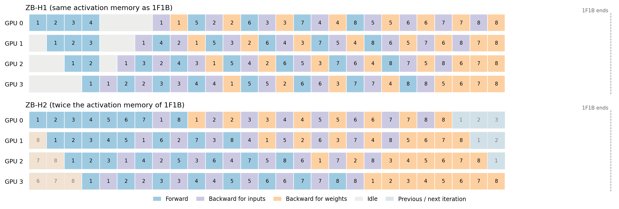
ZB-H1 (top) and ZB-H2 (bottom). Every backward pass is split into a backward for inputs and a backward for weights, and the latter fill the bubbles. Faded cells in ZB-H2 belong to the previous and next iterations, which interlock with the current one when the optimizer step does not synchronize the stages.
ZB-V
The Zero Bubble paper also introduces ZB-V, which places two model chunks on each GPU in a V shape: the model is split into 2p chunks and GPU i holds chunks i and 2p-1-i. A micro-batch goes down the GPUs through the first half of the model and comes back up through the second half. The first and last chunks (embeddings and loss) are both on GPU 0, and no communication is needed at the turn on the last GPU. When the forward, backward for inputs and backward for weights take the same time, ZB-V has zero bubble (again with the optimizer post-validation) with the same peak activation memory as 1F1B, balanced across all GPUs. The price is twice the point-to-point communication of 1F1B. A follow-up paper, Pipeline Parallelism with Controllable Memory (Sea AI Lab, 2024, arXiv), generalizes V-shape schedules to a family that trades bubbles for memory, down to half (V-Half) and a third (V-Min) of the activation memory of 1F1B. ZB-V is available as ScheduleZBVZeroBubble in PyTorch.

ZB-V with 8 model chunks on 4 GPUs. Light cells refer to the first chunk on each GPU (chunks 0 to 3, going down) and dark cells to the second chunk (chunks 4 to 7, going back up). Faded cells belong to the previous and next iterations.
DualPipe
DeepSeek-V3 Technical Report (DeepSeek-AI, 2024, arXiv) introduced DualPipe, later open-sourced in the DualPipe repository. It was designed for Mixture-of-Experts models trained with expert parallelism across nodes, where the all-to-all communication that dispatches tokens to experts and combines their outputs takes roughly as long as the computation itself. The key idea is to overlap the forward pass of one micro-batch with the backward pass of another. Both passes are divided into attention, all-to-all dispatch, MLP and all-to-all combine components (with the backward further split into backward for inputs and backward for weights, as in Zero Bubble). These components are then rearranged, with a manually tuned split of the GPU’s streaming multiprocessors between communication and computation, so that the communication of each pass is hidden behind the computation of the other.
To have enough of these forward-backward pairs, DualPipe uses a bidirectional pipeline: half of the micro-batches enter at the first GPU and flow forward, while the other half enter at the last GPU and flow in the opposite direction. GPU i therefore holds stages i and p-1-i, i.e. two copies of the model parameters, whose gradients are summed across GPUs i and p-1-i before the optimizer step. DeepSeek notes that, in their setup, this duplication does not increase memory significantly, due to the large expert-parallel size. The bubble is (p/2-1)(F&B+B-3W), where F&B is the time of an overlapped forward-backward pair, and each GPU stores the activations of p+1 micro-batches. Compared to Chimera (ETH Zurich, 2021, arXiv), an earlier bidirectional schedule, DualPipe only requires the number of stages and micro-batches to be even (and not the micro-batches to be a multiple of the stages), and its bubble and activation memory do not grow with the number of micro-batches.
Note that our diagrams model only computation, so DualPipe’s bubble looks comparable to ZB-H1’s. Its main advantage is that, within each black-bordered pair, the all-to-all communication of expert parallelism is hidden behind useful computation.

DualPipe on 4 GPUs: micro-batches 1 to 4 (light) enter at GPU 0, and micro-batches 5 to 8 (dark) enter at GPU 3. Each GPU holds two pipeline stages. Cells with a shared black border are the forward and backward passes of two different micro-batches executed together, so that the communication of one overlaps with the computation of the other.
DualPipeV
Sea AI Lab later noticed that DualPipe is made of two mirrored halves, as GPUs i and p-1-i hold the same stages and run the same schedule (DualPipe could be better without the Dual (Sea AI Lab, 2025)). Keeping only the first half of the GPUs and placing the remaining stages on them in a V shape, as in ZB-V, gives a schedule with the same bubble and activation memory as DualPipe for the same number of stages, but on half the GPUs and without duplicated parameters. DeepSeek adopted this cut-in-half schedule as DualPipeV in the DualPipe repository, and recent PyTorch versions provide it as ScheduleDualPipeV. As in ZB-V, all micro-batches enter at GPU 0, go down the GPUs and come back up, and the loss is computed on GPU 0.

DualPipeV with 8 model chunks on 4 GPUs. Light cells refer to the first chunk on each GPU (going down) and dark cells to the second chunk (going back up). Cells with a shared black border are overlapped forward and backward passes of two different micro-batches.
Summary
The table below compares the schedules in the diagrams above (4 GPUs and 8 micro-batches). Idle time is measured in forward passes. Activation memory is measured in activations of one micro-batch on one 1F1B stage, on the GPU that needs the most, assuming the backward for inputs and the backward for weights each release half of a micro-batch’s activations.
| Schedule | Idle time per GPU | Peak activation memory | Parameters per GPU | Main cost |
|---|---|---|---|---|
| 1F1B | 9 | 4 | 1× | - |
| Interleaved 1F1B (2 chunks) | 4.5 | 5.5 | 1× | 2× point-to-point communication |
| ZB-H1 | 3 | 4 | 1× | split backward pass |
| ZB-H2 | 0 (3) | 7.5 | 1× | 2× activation memory, optimizer post-validation |
| ZB-V | 0 (1.5) | 4 | 1× | 2× point-to-point communication, optimizer post-validation |
| DualPipe | 2 | 5 | 2× | duplicated parameters, overlapped forward-backward implementation |
| DualPipeV | 3 | 4.5 | 1× | overlapped forward-backward implementation |
For ZB-H2 and ZB-V, the value in parenthesis is the idle time when the optimizer step synchronizes all stages. DualPipe and DualPipeV also hide the all-to-all communication of expert parallelism behind computation, which is not captured in this table.