Distributed training: sequence and context parallelism with Ulysses and Ring attention
In this post we will discuss and implement context and sequence parallelism, a technique to parallelize computation across the sequence-length dimension. Sequence parallelism is just another possible dimension of model parallelism on the universe of data, tensor, pipeline, tensor, context, sequence and expert parallelism.
Many model inputs and activations include an extra dimension that represents an (un)ordered sequence of tokens. A few examples are temporal datasets with a shape (B, T, E) for text with batch size B, sequence length or token count T and embedding E. Also, videos of shape (B, C, T, H, W) for C channels, T frames, and HxW pixels per frame. And attention scores and probabilities, with shape (B, H, T, T) for H heads and sequences of length T. In these scenarios, we can explore parallelism on the sequence/time dimension T. Following the same notation as text, sequence parallelism requires a local storage of (B, T/P, E) per process. With that in mind, in this post we will implement two existing techniques for sequence parallelism: Ulysses and Ring Attention. Our use case will be a model composed of a sequence of GPTlite blocks, where each block is a multi-head attention (MHA) module followed by a feed-forward network (FFN), with some normalization and skip connections.
Before we continue, we emphasize the following:
- We call our algorithms sequence parallelism even though several sources also use the term context parallelism. In practice, sequence parallelism splits the sequence (token) dimension across GPUs so each device processes a different chunk of tokens, mainly to scale activation memory/compute with longer sequences. Context parallelism splits the attention context (keys/values) across GPUs, so each device holds a slice of the KV context and computes partial attention that’s combined via communication, mainly to scale attention/KV-cache memory for very large context windows. In many scenarios (including this post), we effectively use both: we split the input tokens and also distribute the KV elements needed by attention.
- We focus on training and inference prefill. This is not to be confused with sequence/context parallelism for the inference decode step, which is a different setting: decode processes one token at a time and typically shards the KV cache rather than the input tokens.
Data loader setup for sequence parallelism
To implement sequence parallelism, we first have to adapt our data loader to load data at the token level, in a way that matches our hybrid data- and sequence-parallel setup. All we need to do is configure a DataLoader and DistributedSampler that allocate chunks of sequences (instead of full sequences) to the data loader worker.
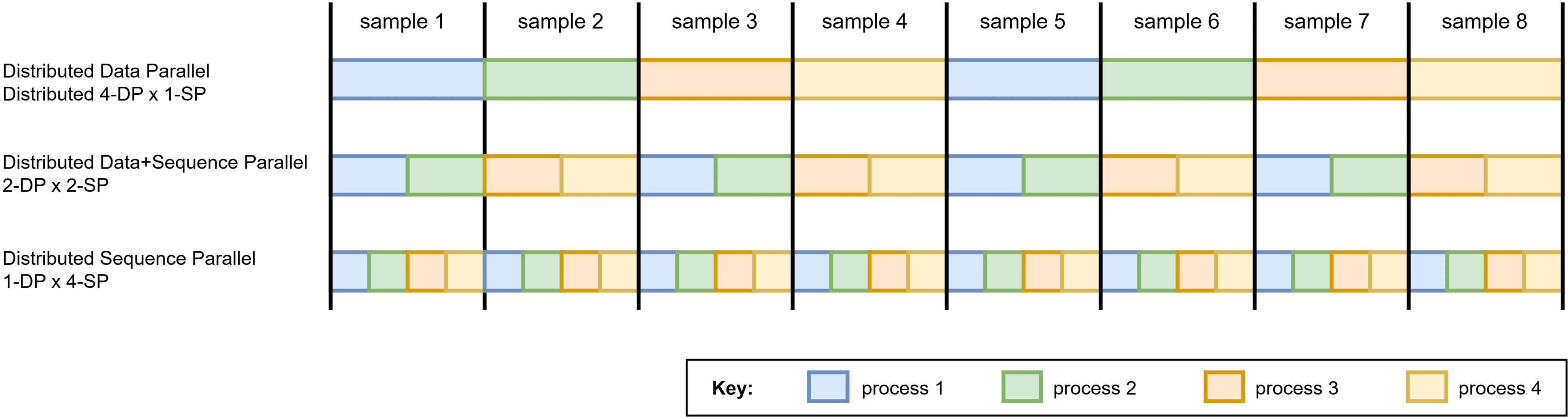
An example of data loading for hybrid parallelism (DP) and sequence parallelism (SP) on 4 processes/GPUs (color-coded), on a dataset of 8 samples. First row: all 4 processes run distributed data parallelism. Second row: creating a custom DistributedSampler that yields chunks of sequences enables a hybrid data- and sequence-parallel execution of 2 groups of 2 sequence-parallel processes. Third row: no data parallelism — all 4 processes execute sequence parallelism on the same sample.
Once this is in place, most layers (like the Feed Forward network) operate across the last/embedding dimension of the input, and are therefore able to run a sequence-parallel train/prefill of the input without changes. The attention layer is an exception, and is covered next.
Distributed attention for context parallelism
During training/inference, the model runtime can scale well with the sequence parallelism degree, except for the attention layer. This is due to the fact that, to reduce activation memory footprint, each GPU only stores a subset of the KV elements.
In practice, to compute the attention module, one process needs its subset/chunk of queries, but needs the keys and values for the full sequence. The rationale is the following: take the attention head computation \(softmax \left(QK^T \right)V\), where all tensors are shaped (B, T, E). If each process holds a subset of rows of \(Q\) as \(Q_p\) with shape (B, T/P, E), it needs to access all elements of \(K^T\) and \(V\) to be able to perform the dot-product \(Q_p K^T\), the row-wise \(softmax\), and the dot-product by \(V\), resulting in the attention output per process of shape (B, T/P, E):
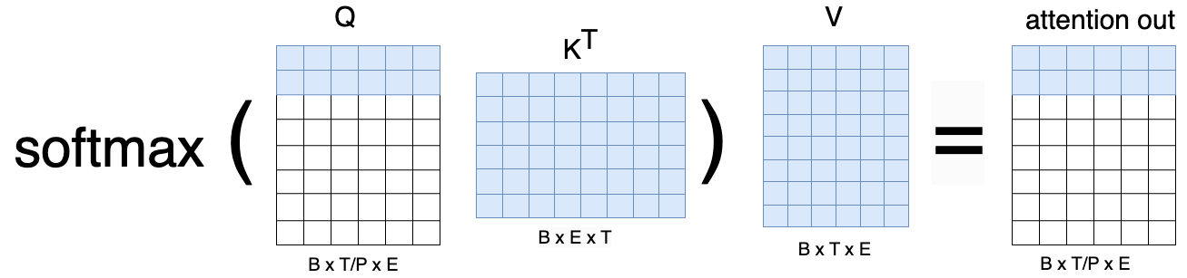
Therefore, sequence parallelism requires some communication to make the relevant KV elements accessible across all GPUs. With that in mind, in the following sections we will look into two alternative algorithms for sequence/context parallel attention.
Ulysses sequence parallelism
Take the previous notation and assume a mini-batch split across the time dimension, with a local storage of (B, T/P, E) per process.
If we pass such a shape to a feed-forward network, we achieve parallelism of order P, as the T dimension will be treated as batch by the linear layers. However, in the case of multi-head attention, there is a need for process communication because time dependencies across the tokens require access to the full attention context.
(DeepSpeed) Ulysses parallelism solves this by swapping the distributed view from time-split to head-split before and after the MHA module, as in the following illustration:
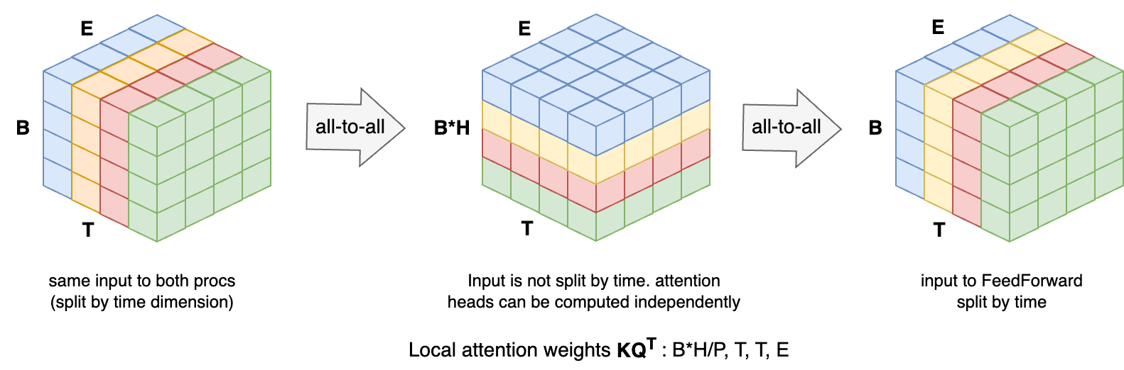
Overview of Ulysses sequence parallelism. Left: the initial view of the input tensor, distributed across 4 (color-coded) GPUs, split by the time (T) dimension. Center: the first all-to-all changes the distributed tensor view from time- to head-split. Each process now holds complete sequences (i.e., not time-split) for a subset of heads and can compute attention locally. Right: the second all-to-all reverts the view from head- to time-split.
In practice, the implementation of Ulysses only requires extra steps that swap the distributed view of the input tensor from e.g. (H, B, T/P, E) to (H/P, B, T, E) and vice-versa. We can implement a function dist_view_swap() that, given a tensor whose sequence is distributed across the process group group, swaps the distributed view by changing the split dimension from old_split_dim to new_split_dim:
def dist_view_swap(tensor: torch.Tensor, old_split_dim: int, new_split_dim: int, group: dist.ProcessGroup):
    '''Swap the distributed split dimension of a tensor of local shape (H, B, T/P, E) across P processes.'''
    full_shape, P = list(tensor.shape), group.size()
    full_shape[old_split_dim] *= P  # full distributed shape
    H, B, T, E = full_shape

    send = torch.cat([tensor.chunk(P, dim=new_split_dim)[r].contiguous() for r in range(P)])
    recv = torch.zeros_like(send)
    dist.all_to_all_single(output=recv, input=send, group=group)

    recv = torch.cat(
        [recv.chunk(P)[r].view(H // P, B, T // P, E) for r in range(P)],
        dim=old_split_dim,
    )
    return recv
From here, the implementation is straightforward. The first (leftmost) all-to-all in the Ulysses diagram above converts the distributed view from time-split to head-split, while the backward pass does the inverse view swap:
class first_alltoall(torch.autograd.Function):

    @staticmethod
    def forward(ctx, x, group=None):
        ctx.group = group  # save for backward pass
        return dist_view_swap(x, old_split_dim=2, new_split_dim=0, group=ctx.group)

    @staticmethod
    def backward(ctx, dout):
        dout = dist_view_swap(dout, old_split_dim=0, new_split_dim=2, group=ctx.group)
        return dout, None
The second all-to-all is analogous, except that it performs the opposite view changes in the forward and backward passes:
class second_alltoall(torch.autograd.Function):

    @staticmethod
    def forward(ctx, x, group=None):
        ctx.group = group
        return dist_view_swap(x, old_split_dim=0, new_split_dim=2, group=ctx.group)

    @staticmethod
    def backward(ctx, dout):
        dout = dist_view_swap(dout, old_split_dim=2, new_split_dim=0, group=ctx.group)
        return dout, None
Now we can implement the MultiHeadAttention module by calling both all-to-alls as modules:
from flash_attn.flash_attn_interface import flash_attn_func

class MultiHeadAttention(nn.Module):

    def __init__(self, n_embd=256, d_head=128, n_heads=8, dropout_p=0.1, group=None):
        '''An Ulysses multi-head attention. Variable names follow GPTlite's post.'''

        super().__init__()
        self.d_head = d_head
        self.n_heads = n_heads
        self.keys = nn.ModuleList([nn.Linear(n_embd, d_head, bias=False) for _ in range(n_heads)])
        self.queries = nn.ModuleList([nn.Linear(n_embd, d_head, bias=False) for _ in range(n_heads)])
        self.values = nn.ModuleList([nn.Linear(n_embd, d_head, bias=False) for _ in range(n_heads)])
        self.proj = nn.Linear(n_heads * d_head, n_embd)
        self.dropout = nn.Dropout(dropout_p)

        self.group = group  # Ulysses group
        if self.group is None:
            self.group = dist.new_group(range(dist.get_world_size()))

    def forward(self, x):
        # x is local chunk: (B, T/P, E)
        P = self.group.size()
        B, T_local = x.shape[0], x.shape[1]
        T = T_local * P

        # Q, K and V embeddings: (B, T/P, E) -> (H, B, T/P, d_head)
        q = torch.stack([q(x) for q in self.queries], dim=0)
        k = torch.stack([k(x) for k in self.keys], dim=0)
        v = torch.stack([v(x) for v in self.values], dim=0)

        if P > 1:  # (H, B, T/P, d_head) -> (H/P, B, T, d_head)
            q = first_alltoall.apply(q, self.group)
            k = first_alltoall.apply(k, self.group)
            v = first_alltoall.apply(v, self.group)

        # flash_attn expects (B, T, H_local, d_head)
        q_ = q.permute(1, 2, 0, 3)
        k_ = k.permute(1, 2, 0, 3)
        v_ = v.permute(1, 2, 0, 3)

        dropout_p, softmax_scale = 0.0, q_.shape[-1] ** (-0.5)
        out = flash_attn_func(q_, k_, v_, dropout_p, softmax_scale)  # (B, T, H/P, d_head)

        out = out.permute(2, 0, 1, 3)  # (H/P, B, T, d_head)

        if P > 1:  # (H/P, B, T, d_head) -> (H, B, T/P, d_head)
            out = second_alltoall.apply(out, self.group)

        out = out.permute(1, 2, 0, 3)  # (H, B, T/P, d_head) -> (B, T/P, H, d_head)
        out = out.reshape(B, T // P, -1)  # (B, T/P, H, d_head) -> (B, T/P, H*d_head)
        out = self.proj(out)  # (B, T/P, H*d_head) -> (B, T/P, E)
        out = self.dropout(out)
        return out
And that is it. It’s conceptually simple, and the full implementation can be found in gptlite_ulisses_sequence_parallelism.py.
As an important note, there are other similar approaches to handle this problem, such as ColAI-SP and Megatron-SP. The big advantage of DeepSpeed Ulysses parallelism is that it requires less communication than the alternatives. The main downsides are that the maximum parallelism is dictated by the number of attention heads (typically 8), and that the all-to-all requires blocking collective communication that may incur heavy overhead on slow interconnects. That’s where Ring Attention comes into play.
Ring Attention
Ring attention was presented in the paper Ring Attention with Blockwise Transformers for Near-Infinite Context, building on Blockwise Parallel Transformer for Large Context Models. It performs a per-block computation of attention that allows one to compute \(softmax \left(QK^T \right)V\) without materializing the full attention matrix or requiring all keys/values to be present at once. It can be viewed as a distributed variant of Flash Attention. The core rationale is also related to the ideas in Self-attention Does Not Need \(O(n^2)\) Memory.
Given scores \(s_i = dot(q, k_i)\) for a single query row, the attention output can be written as:
\[\text{Attention}(q, K, V) = \sum_i \text{softmax}(s)_i \, v_i = \sum_i \left( \frac{\exp(s_i)}{\sum_j \exp(s_j)} \right) v_i = \frac{\sum_i \exp(s_i)\, v_i}{\sum_j \exp(s_j)}.\]This formulation exposes that the output is a fraction whose numerator and denominator are sums of terms. Therefore, we do not need to store the full attention matrix \(QK^T\). Instead:
- In the forward pass, we iterate over blocks of keys/values and accumulate \(v^{\star} \leftarrow v^{\star} + \exp(s_i)\, v_i\) (numerator) and \(s^{\star} \leftarrow s^{\star} + \exp(s_i)\) (denominator);
- After processing all keys and values, we divide \(\frac{v^{\star}}{s^{\star}}\) to get the final attention output;
- In the backward pass we compute gradients blockwise, therefore not needing to store the whole attention matrix from the forward pass.
Improving numerical stability
The previous formulation is not numerically stable in floating point arithmetic because the softmax exponents can lead to very large numbers. A standard solution is to compute softmax by subtracting the maximum score from all scores. This does not change the result of the softmax but avoids overflow/underflow. This is called the safe softmax trick and is well explained in this post. The safe softmax formulation is:
\[safe\_softmax(s_i) = \frac{\exp (s_i - s_{max})}{ \sum_j \exp( s_j - s_{max})}.\]The issue is how to compute the max value when the computation is done in blocks. This is done by keeping the max value of all blocks seen so far in the iterative loop over blocks. Then, if the current maximum at block \(j\) is \(m_j\) and the previous maximum value until then was \(m_{j-1}\), the accumulators are updated as:
\[\begin{align*} v^{\star} \leftarrow & \, v^{\star} \cdot \exp ( m_{j-1} - m_{j}) + \exp \left( s_j- m_{j} \right) \, v_j \\ s^{\star} \leftarrow & \, s^{\star} \cdot \exp( m_{j-1} - m_{j} ) + \exp \left( s_j- m_{j} \right). \end{align*}\]Finally, in practice we often do not compute \(v^{\star}\) and \(s^{\star}\) directly, but apply a small variation where we accumulate log-values (LogSumExp / LSE) for better stability (described here ), due to the LSE property:
\[LSE (x_{1},\dots ,x_{n})=\log \left(\exp(x_{1})+\cdots +\exp(x_{n})\right).\]Distributed algorithm
Now that we know how to compute the attention output per block, we can parallelize attention by delegating a sub-block to each processor. We start with sequence parallelism of the tensors \(q\), \(k\) and \(v\) across \(P\) processes, i.e., each process holds a non-overlapping time block of the \(q\), \(k\) and \(v\) tensors. Just like Ulysses, this allows for direct P-order parallelism on the feed-forward network, but not on multi-head attention.
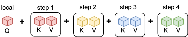
During ring attention, each process keeps its local chunk of queries, and rotates the key/value blocks among all \(P\) processes in a ring fashion: at each communication step (out of \(P\) steps), each process sends its block of keys/values to the next process and receives the keys/values block from the previous process in the ring. After \(P\) steps, every process has seen all key/value blocks and can compute attention for its local queries.
This pattern can be illustrated as:
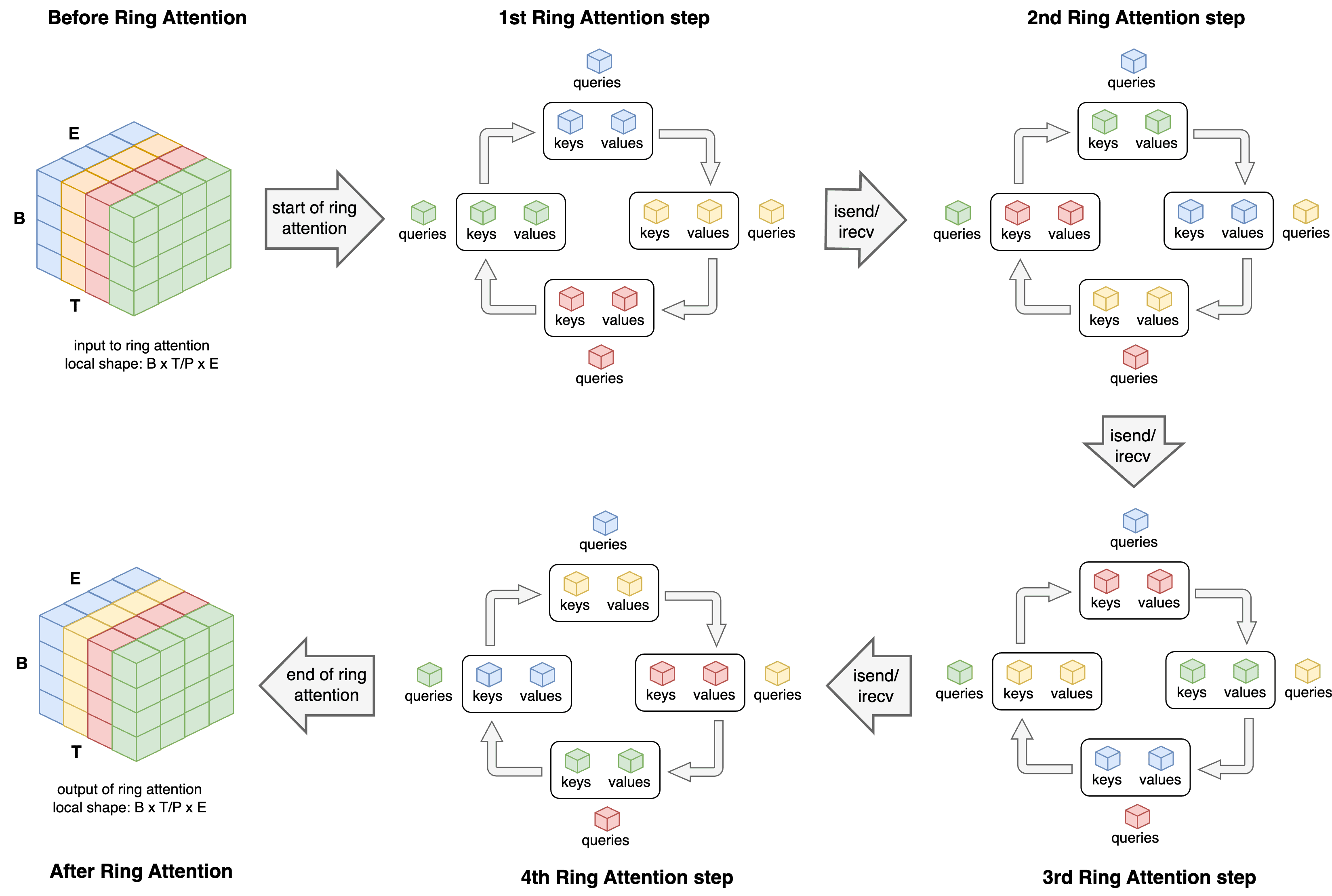
Overview of the Ring Attention algorithm. Before Ring Attention: the initial view of the input tensor, distributed across 4 (color-coded) GPUs, split by the time (T) dimension. 1st Ring Attention step: each process holds its part of the Query, Key and Value tensors and computes block attention for those tensors. Asynchronously, processes send the Key and Value tensors to the next process in the ring (clockwise). 2nd, 3rd, and 4th steps: each process receives the previous process’ Key and Value blocks and computes attention output for its original Query tensor and the received Key/Value tensors. After Ring Attention: the MHA output is already time-split across processes, similarly to the initial data format.
From a process standpoint, after all ring steps, each process has its own time block of \(q\) and has iterated over the full \(k\) and \(v\) tensors (in chunks). As an example, for the third (red) process above, we’d have the following data presented:
A very relevant mention is that while Ulysses performs communication synchronously (all-to-all), forcing processes to wait for communication to complete, ring attention can use asynchronous point-to-point communication. If the computation time of a block exceeds the transmission time, communication overhead can be masked by computation.
Implementation
The forward pass performs \(P\) ring communication steps, and on each step it computes attention output and the per-row LogSumExp (variables block_out and block_lse) in order to do the accumulation:
import flash_attn.flash_attn_interface as fa  # flash attention

class RingAttention(torch.autograd.Function):

    @staticmethod
    def forward(ctx, q, k, v, group):

        P = group.size()
        q, k, v = q.contiguous(), k.contiguous(), v.contiguous()  # (B, T/P, H, E)

        out = lse = None  # accumulators
        recv_k, recv_v = torch.empty_like(k), torch.empty_like(v)  # recv buffers

        for step in range(P):  # do P ring steps

            # send K and V for next step, asynchronously
            reqs_k_v = isend_k_and_v(k, v, recv_k, recv_v, group)

            # compute attention output and softmax lse for current block
            dropout_p, softmax_scale = 0.0, q.shape[-1] ** (-0.5)
            kwargs = dict(causal=False, window_size=(-1, -1), softcap=0.0, alibi_slopes=None, return_softmax=False)
            block_out, _, _, _, _, block_lse, _, _ = fa._flash_attn_forward(q, k, v, dropout_p, softmax_scale, **kwargs)

            # update out and lse
            out, lse = accumulate_out_and_lse(out, lse, block_out, block_lse)

            # wait for new K and V before starting the next iteration
            [req.wait() for req in reqs_k_v]
            k, v = recv_k, recv_v

        ctx.group = group  # save for backward
        out = out.to(dtype=q.dtype)
        ctx.save_for_backward(q, k, v, out, lse)
        return out
where isend_k_and_v(k, v, recv_k, recv_v, group) is the function that sends the tensors k and v to the next neighbour asynchronously, receives the previous neighbour’s k and v into recv_k and recv_v asynchronously, and returns the send/receive communication futures that have to be waited on with req.wait().
The backward pass takes as input the gradient of the loss with respect to the output (\(\nabla_{out} Loss\) or dout in the code below), and returns the gradients with respect to the inputs (gradients \(\nabla_{q} Loss\), \(\nabla_{k} Loss\), \(\nabla_{v} Loss\), or dq, dk, dv):
    @staticmethod
    def backward(ctx, dout, *args):

        P = ctx.group.size()
        q, k, v, out, softmax_lse = ctx.saved_tensors
        softmax_lse = softmax_lse.squeeze(dim=-1).transpose(1, 2)

        block_dq = torch.empty_like(q)
        block_dk = torch.empty_like(k)
        block_dv = torch.empty_like(v)

        dq = torch.zeros_like(q)
        dk = torch.zeros_like(k)
        dv = torch.zeros_like(v)

        recv_k, recv_v = torch.empty_like(k), torch.empty_like(v)
        recv_dk, recv_dv = torch.empty_like(dk), torch.empty_like(dv)

        for step in range(P):

            # send K and V for next step, asynchronously
            reqs_k_v = isend_k_and_v(k, v, recv_k, recv_v, ctx.group)

            # compute gradients for the current block K/V and local Q
            dropout_p, softmax_scale = 0.0, q.shape[-1] ** (-0.5)
            kwargs = dict(causal=False, window_size=(-1, -1), softcap=0.0, alibi_slopes=None,
                          deterministic=False, rng_state=None)
            fa._flash_attn_backward(
                dout, q, k, v, out, softmax_lse,
                block_dq, block_dk, block_dv,
                dropout_p, softmax_scale, **kwargs
            )

            if step > 0:
                # wait for dK and dV from the previous steps (rotated accumulators)
                [req.wait() for req in reqs_dk_dv]
                dk, dv = recv_dk, recv_dv

            dq += block_dq
            dk += block_dk
            dv += block_dv

            # rotate dK and dV alongside K and V
            reqs_dk_dv = isend_k_and_v(dk, dv, recv_dk, recv_dv, ctx.group)

            # wait for new K and V before the next iteration
            [req.wait() for req in reqs_k_v]
            k, v = recv_k, recv_v

        # before returning, wait for the last dK and dV for this process' original block
        [req.wait() for req in reqs_dk_dv]
        dk, dv = recv_dk, recv_dv
        return dq, dk, dv, None
A nuance in the backward pass is that the gradients of a given block refer to the current \(K\) and \(V\) which are being rotated around processes. Therefore, the gradients dk and dv are also accumulated by being rotated alongside their k and v blocks.
Finally, the forward pass of multi-head attention is straightforward and simply calls ring attention instead of regular attention:
class MultiHeadAttention(nn.Module):
     def forward(self, x):
        P = self.group.size()
        B, T_local = x.shape[0], x.shape[1]
        T = T_local * P

        # take Q, K and V, and collect all head embeddings: (B, T/P, E) -> (H, B, T/P, E)
        q = torch.stack([q(x) for q in self.queries], dim=0)
        k = torch.stack([k(x) for k in self.keys], dim=0)
        v = torch.stack([v(x) for v in self.values], dim=0)

        # convert to flash-attn layout (B, T/P, H, E)
        q_ = q.permute(1, 2, 0, 3)
        k_ = k.permute(1, 2, 0, 3)
        v_ = v.permute(1, 2, 0, 3)

        if P == 1:
            out_ = fa.flash_attn_func(q_, k_, v_)
        else:
            out_ = RingAttention.apply(q_, k_, v_, self.group)

        out = out_.reshape(B, T // P, -1)  # (B, T/P, H, E) -> (B, T/P, H*E)
        out = self.proj(out)  # (B, T/P, H*E) -> (B, T/P, E)
        out = self.dropout(out)
        return out
And we are done. As we can see, a key disadvantage in ring attention is that the number of communication steps equals the number of processes. This may be a limiting factor on large networks where very fine-grained sequence splits lead to small per-process workloads, making it harder to fully hide communication with computation.
This code has been added to the GPTlite-distributed repo. Keep in mind that deterministic behaviour for sequence parallelism across networks of different node counts is difficult due to random number generators producing different values during model initialization and dropout.
When to use Ulysses and Ring attention
Use Ulysses when the group sits on a fast interconnect like NVLink within a node and the degree is less-or-equal than the number of attention heads. That means we cannot use Ulysses with Multi-Query Attention (MQA), and it has limited use on Grouped Query Attention (GQA). A benefit of Ulysses is that any attention kernel works unchanged, and woks well for any mask. However, the disadvantage is that the all-to-all is hard to overlap with compute and slows down across nodes.
Use Ring attention when we need a degree beyond the head count or across nodes. It has no head limit and hides communication, but only if each local chunk is long enough for compute to cover the transfer. However, Ring Attention is not ideal for any custom or arbitrary attention mask: while the fundamental blockwise formulation can mathematically support any masking pattern, its real-world implementation depends on overlapping communication with computation (so the mask should ideally yield computation on each step). In practice, most standard Ring Attention libraries natively support only causal masks (triangular masks used in autoregressive models) or general/document masks (unmasked bidirectional attention). To overcome this, variants like Striped Attention and Llama 3 Zigzag Ring Attention explicitly permute and optimize data chunks around the specific mathematical structure of a causal mask to balance the hardware workload.
Both methods have drawbacks. The rule of thumb is to use a hybrid algorithm once we span multiple nodes: Ulysses inside each node and Ring across nodes, which usually beats either alone at scale. Hybrid algorithms for sequence parallelism are also discussed in USP: A Unified Sequence Parallelism Approach for Long Context Generative AI, LoongTrain: Efficient Training of Long-Sequence LLMs with Head-Context Parallelism, and Megatron’s a2a+p2p for Hierarchical Context Parallelism (HCP, where p2p is ring-exchange and a2a is ulysses-style parallelism).
Training with sequence- and multi-dimensional parallelism
PyTorch does not have the notion of partial sequences in the same way data parallelism has a notion of partial batches. Thus, samples processed in parallel are usually assumed to be full-length samples on a data-parallel execution. To overcome this, when we run sequence parallelism of order S, we must perform S gradient accumulation steps with the corresponding gradient scaling so that we effectively process the intended batch size and gradients are properly averaged.
Moreover, when we perform multi-dimensional parallelism (e.g. data + sequence), we need to define process groups for the data-parallel processes (the ones that load different samples) and the sequence-parallel processes (the ones that load different chunks of the same sample). We can do this with PyTorch’s DeviceMesh or create oue own process groups manually. For the sake of illustration, if we’d implement a \(2 \times 2\) data- and Ulysses sequence parallelism on 4 GPUs, this would be the memory layout before and during the multi-head attention:
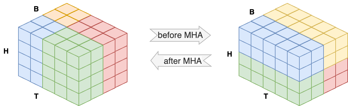
Activations allocation on a 4-GPU execution with 2-GPU data parallelism and 2-GPU Ulysses sequence parallelism. Left: blue and green processes belong to the same sequence-parallel group and share one sample; red and yellow processes form the other sequence-parallel group and share the other sample. Right: the first all-to-all in Ulysses parallelism converts token-level distributed storage into head-level distributed storage. All four processes can compute attention for full sequences.