Distributed Load Balancing and Spatial Slicing
Domain decomposition (or spatial decomposition) divides the objects of a multidimensional space across compute nodes, so that each node gets the same number of objects, close to each other. As objects interact mostly with their neighbors, compact regions, close to squares in 2D or cubes in 3D, need the least communication between nodes. They also cut the fewest objects with volume, which are duplicated on both sides of a boundary. This post compares the simplest spatial decompositions, and details a distributed algorithm for the most efficient of them.
Slicing Layouts
The simplest spatial decomposition algorithms perform an orthogonal spatial decomposition (slicing): every cut is orthogonal to one axis, so that each slice is an axis-aligned rectangle (a box in 3D). In a 2D space, there are several slicing alternatives, numbered 1 to 4 from left to right:
Single Axis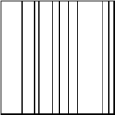 Non-Uniform Grid
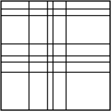 Orthogonal Recursive Bisection
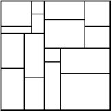 Sort Tile Recursive
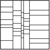
Slicing layout 1 incurs a lot of object duplication when objects are not points in space but have volume, and when there is a high number of slices, as each slice adds a cut across the whole space. Layout 2, the non-uniform grid (NUG), works better by reducing cloning, yet it does not guarantee an accurate spatial decomposition, as the cuts of each dimension are shared by all slices, which may then hold different numbers of objects.
Layout 3 is the orthogonal recursive bisection (ORB), used to balance the work of nonuniform problems on multiprocessors. Layout 4 is the sort tile recursive (STR) layout, used to pack the R-trees of spatial databases. STR sorts the objects on the first axis and cuts them into \(S_1\) slices with the same number of objects. It then sorts the objects of each slice on the second axis and cuts the slice into \(S_2\) slices, and so on for each dimension.
Layouts 3 and 4 are similar, but layout 4 outperforms layout 3 in parallelism. This is because layout 3 performs a tree-based recursive bisectional decomposition (i.e. at every level of the tree it computes 2 slices), while layout 4 performs several slices at once for each of the 2 dimensions. The cuts of layout 3 are those of a balanced k-d tree, which cuts each region in two at the median of its points, along the axes in turn.
The following table details the complexity of each algorithm for \(n\) objects, \(s\) slices and \(d\) dimensions (assuming sorting with an average complexity of \(n \log n\)):
| Scheme | Computation steps | Properties / Limitations |
|---|---|---|
Single Axis |
\(= n \cdot \log_2 n\) | One sorting of all elements on a single direction, independently of the number of dimensions. |
Non-Uniform Grid |
\(= d \cdot n \cdot \log_2 n\) | One sorting of all elements applied to each dimension, iteratively; slicing configuration for the \(d\) dimensions must decompose final number of slices \(s\) i.e. \(\prod_{k=1}^d S_k = s\). |
Sort Tile Recursive |
\(\begin{array}{l} = n \cdot \log_2 n \\ +n \cdot \log_2 \frac{n}{S_1} \\ +n \cdot \log_2 \frac{n}{S_1 S_2} \\ +... \\ +n \cdot \log_2 \frac{n}{S_1 S_2 ... S_{d-1}} \\ = \sum_{i=1}^d n \cdot \log_2 \frac{n}{\prod_{k=0}^{i-1} S_k} \end{array}\) | One sorting for each subslice’s data on each dimension, applied iteratively; sub-slices computations are independent; slicing configuration for the \(d\) dimensions must decompose final number of slices \(s\) i.e. \(\prod_{k=1}^d S_k = s\); Faster than NUG as each new dimension requires sorting across smaller datasets; the sum assumes \(S_0 = 1\) i.e. the initial universe is a single slice including all elements. |
Orthogonal Recursive Bisection |
\(\begin{array}{l} = n \cdot \log_2 n \\ +n \cdot \log_2 \frac{n}{2} \\ +n \cdot \log_2 \frac{n}{4} \\ +n \cdot \log_2 \frac{n}{8} \\ +... \\ +n \cdot \log_2 \frac{n}{s/2} \\ = \sum_{i=1}^{\log_2 s} n \cdot \log_2 \frac{n}{2^{i-1}} \end{array}\) | Total number of slices \(s\) must be a power of 2; requires, at every iteration, one sorting of each slice, which holds half of the elements of its parent slice, for a total of \(\log_2 s\) steps, therefore a slow method on large networks; sub-slices computations are independent. |
Across these four slicing layouts, layout 4 is the most efficient: it guarantees low data duplication, allows for accurate slicing, and requires only \(d\) (dimensions) recursive iterations, regardless of the number of compute nodes (unlike layout 3). However, its implementation in a distributed memory environment is not trivial, as no compute node can hold or sort all the objects. Possible options are:
- A histogram/binning algorithm that clusters elements in spatial bins and uses the number of elements per bin as the metric for slicing;
- A method that performs serial slicing on one compute node that holds only a sample of the data, and uses the slicing of the sampled dataset as the slicing of the final dataset.
Both options are approximate: the bins and the sample only estimate where the cuts fall, so the slices hold about the same number of objects, but not exactly the same.
Distributed Slicing via Sort-Balance-Split
A technique published by the author, called the Sort-Balance-Split (SBS), implements a parallel multi-dimensional slicing based on layout 4. The algorithm follows three steps:
- The sorting step performs a distributed sort of all elements on a given dimension (the implementation uses a distributed sample sort);
- The load balancing step equalizes the number of elements across compute nodes, which the sort leaves uneven, while respecting the initial sorting. Each rank shares its element count with all the others, and computes from the counts the global position of its elements in the sorted order. It then sends each element to the rank that holds this position after the balance, as illustrated in the following picture:
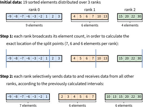
Load balancing of 19 sorted elements on 3 ranks, colored by rank. The first 19 mod 3 = 1 rank holds one more element.
- The splitting step creates smaller networks, called subnetworks, from subsets of consecutive ranks of the main network. In MPI, each subnetwork is a new communicator, a group of ranks with its own collective calls, so that the subnetworks of a level work in parallel. The split is illustrated in the following picture:
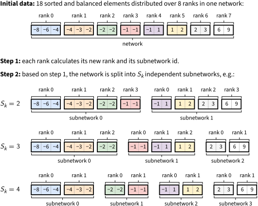
The split of 8 ranks into \(S_k = 2\), \(S_k = 3\) and \(S_k = 4\) subnetworks of consecutive ranks, after the sort and the balance, colored by rank. The data stays in place, and each rank gets a new rank in its subnetwork. For \(S_k = 3\), which does not divide the number of ranks, the subnetworks have 3, 3 and 2 ranks.
The three steps explain the name Sort-Balance-Split. The SBS algorithm is performed recursively at every level, where each level operates on the subnetworks created by the split step of the previous level. Level \(k\) sorts on dimension \(k\) and splits each subnetwork into \(S_k\) subnetworks, so that after the \(d\) levels each rank holds one slice, and \(s = p = S_1 S_2 \cdots S_d\). By default, the implementation picks the \(S_k\) with the smallest sum, such as \(2 \times 2 \times 2\) for 8 ranks and \(16 \times 16 \times 16\) for 4,096 ranks. For objects spread uniformly in a cube, the total area of the cuts is \(S_1 + S_2 + S_3 - 3\) times the area of a face, so the smallest sum gives the least duplication.
Each level needs eight collective calls for its three steps. The distributed sample sort makes four: the gather of the samples, the broadcast of the splitters, and the all-to-all exchanges of the counts and of the elements. The balance makes three: the all-gather of the counts, and the all-to-all exchanges of the send counts and of the elements. The split makes one. This number does not depend on the number of objects, so that a 3D slicing takes 24 collective calls. On large networks, the implementation gathers the samples in two stages, so that no rank receives all the \(p(p-1)\) samples, at the cost of a few more calls per level.
This method has two advantages over existing methods: (1) a fixed number of communication steps, for any network size, input size and distribution of the data; and (2) an accurate spatial decomposition, i.e. not an approximation. However, SBS moves the objects at every level, and most of them change rank at each level when they are placed at random. The histogram and sampling methods compute an approximate slicing first and then move each object only once: these are preferable when an approximate balance is enough.
A sample application of the algorithm on a 2D universe of 16 shapes distributed across 4 compute nodes (ranks) is presented below:
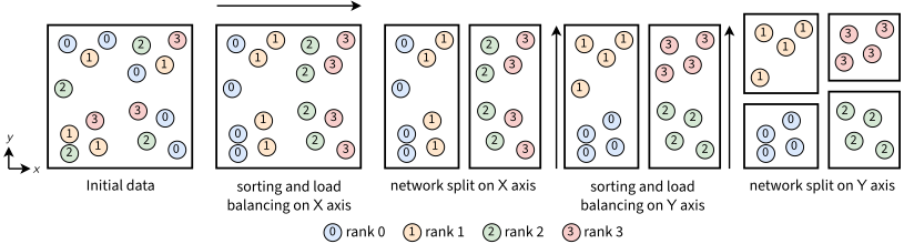
From left to right:
- Initial data layout;
- The initial sorting operation sorts all elements on the first (X) dimension, without caring about the other coordinates. Data is load balanced on the X axis, so that each rank holds 4 shapes;
- A network split divides the initial problem of 16 shapes across 4 nodes on a single network into 2 problems of 8 shapes, each on a subnetwork of 2 nodes;
- Each subnetwork performs a distributed sort of its objects on the next axis (Y), and balances the workload;
- A network split on the Y axis gives the final data layout, where each rank holds one slice of 4 shapes.
Here is another illustration of the same problem in a 3D universe, now emphasizing the memory layout across nodes:
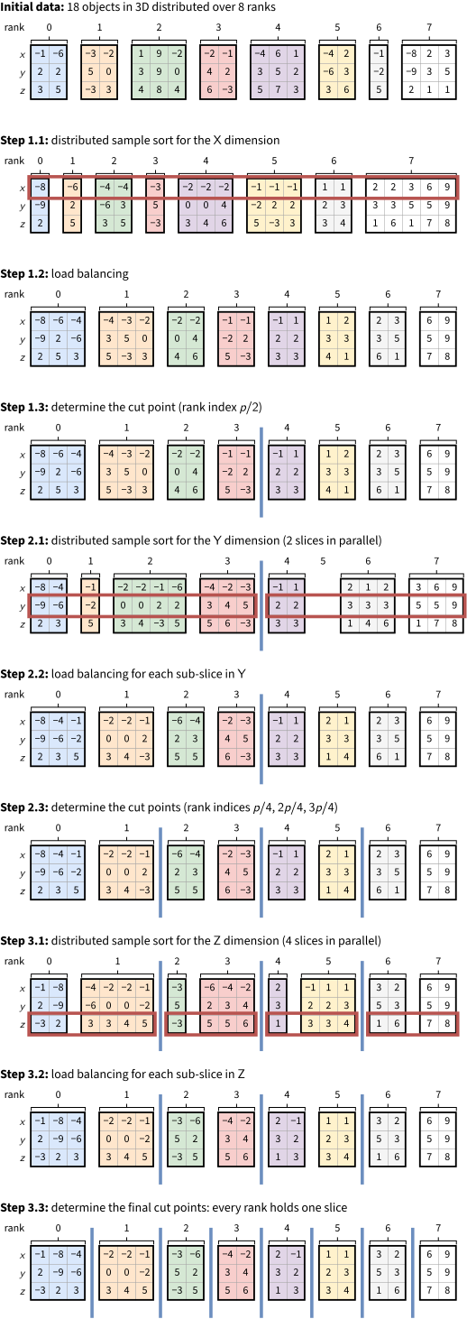
Sort-Balance-Split of 18 objects in 3D on \(p = 8\) ranks, with \(S_1 = S_2 = S_3 = 2\), colored by rank. Each column is one object, with its coordinates \(x\), \(y\) and \(z\). Red frames mark the coordinate that steps 1.1, 2.1 and 3.1 sort in each slice, and blue lines the cuts between the subnetworks. In step 2.1, two splitters of the second subnetwork are equal, so rank 5 receives no object until the balance.
And here is an application of distributed slicing to the N-body problem (left), which simulates the formation of cosmic structures after the Big Bang. The picture on the right shows the slicing of a small network of neurons:
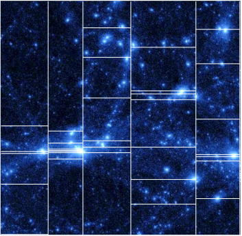
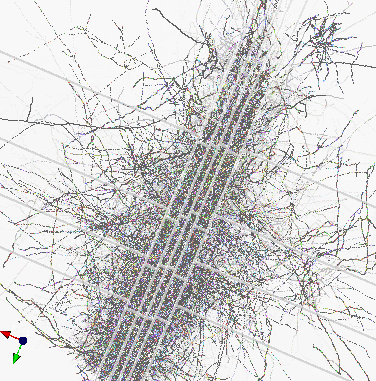
For further reading, our original paper details SBS and evaluates it on 4,096 nodes of an IBM Blue Gene/Q supercomputer, with up to a trillion elements. There, it scales almost linearly, and it gives a better load balance in a shorter time to solution than the sampling and parallel partitioning methods of its time.
The C++ implementation, with MPI, is available in slicing.tar.gz.