Unsupervised Learning for Dimensionality Reduction (PCA)
This post continues the post on clustering with the other main task of unsupervised learning. Dimensionality reduction maps the data to fewer dimensions that keep most of its structure, to compress it, to visualize it in 2D or 3D, or to prepare it for other methods, such as clustering. PCA and kernel PCA keep the directions of largest variance, t-SNE keeps the neighbors of each point, and ICA finds the directions of independent signals. Each of them comes with a short NumPy implementation.
Principal Component Analysis
Principal Component Analysis (PCA) rotates the data towards the directions of largest variance, so that the data can be analyzed along its most meaningful dimensions, and the dimensions of low variance discarded. For \(n\) data points \(x_1, ..., x_n\), the algorithm is the following:
- center the data by subtracting the mean: \(x_i \leftarrow x_i - \bar{x}\), with \(\bar{x} = \frac{1}{n} \sum_{i=1}^n x_i\);
- compute the covariance matrix of the centered data: \(C = \frac{1}{n-1} \sum_{i=1}^n x_i \, x_i^{T}\);
- compute the eigenvalues \(\lambda_i\) and eigenvectors \(v_i\) of the covariance matrix, i.e. the solutions of \(C v_i = \lambda_i v_i\). Each eigenvalue is the variance of the data along its eigenvector;
- build the feature matrix \(F\), whose columns are the eigenvectors in the order of decreasing eigenvalues;
- the transformed data is the product of the transposed feature matrix and the matrix \(D_c\) whose columns are the centered data points: \(D_n = F^T D_c\).
A visual example is displayed below, where PCA rotates the data towards the new axes of the cluster of data points:
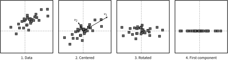
1. Points of a 2D Gaussian. 2. The centered data, and the eigenvectors \(v_1\) and \(v_2\) of its covariance matrix, scaled to three standard deviations of the data along them. 3. The transformed data \(D_n = F^T D_c\): the rotation turns \(v_1\) to the horizontal axis and \(v_2\) to the vertical axis. 4. The first principal component only: each point is described by one number. Inspired by: Principal component analysis
The least significant dimensions of the transformed data can now be discarded. The number of eigenvectors kept in \(F\) sets the compression: the first \(k\) components explain a fraction \(\sum_{i=1}^k \lambda_i / \sum_{i} \lambda_i\) of the variance of the data, a common criterion to choose \(k\).
To recover the original data, the transformation is inverted. The eigenvectors of the symmetric matrix \(C\) are orthonormal, so \(F^T F = I\), and the centered data is given by \(D_c = F D_n\), to which the mean \(\bar{x}\) is added back. When \(F\) keeps only \(k\) eigenvectors, \(F D_n\) is the best approximation of \(D_c\) by \(k\) dimensions, in the least-squares sense.
PCA can be implemented as:
def pca(X, k):
    Xc = X - X.mean(0)  # the centered data, one point per row
    C = Xc.T @ Xc / (len(X) - 1)  # the covariance matrix
    lam, F = np.linalg.eigh(C)  # its eigenvalues, in increasing order, and eigenvectors
    F = F[:, ::-1][:, :k]  # the k eigenvectors of largest eigenvalues
    return Xc @ F  # the transformed data D_n = F^T D_c, one point per row
Kernel PCA
PCA only finds linear structure. Kernel PCA applies PCA in a high-dimensional feature space \(\phi(x)\), where the non-linear structure of the input space may become linear. The kernel trick avoids computing \(\phi\), as the method only needs the dot products \(k(x_i, x_j) = \phi(x_i)^T \phi(x_j)\), given by a kernel function such as the Gaussian kernel \(k(x_i, x_j) = \exp \left( - \| x_i - x_j \|^2 / 2 \sigma^2 \right)\). The algorithm is:
- compute the \(n \times n\) kernel matrix \(K\), with \(K_{ij} = k(x_i, x_j)\);
- center the data in the feature space: \(\tilde{K} = K - 1_n K - K 1_n + 1_n K 1_n\), where \(1_n\) is the \(n \times n\) matrix with all entries equal to \(1/n\);
- compute the eigenvalues \(\lambda_m\) and eigenvectors \(\alpha^{(m)}\) of \(\tilde{K}\), and scale each eigenvector so that \(\lambda_m \, \alpha^{(m)T} \alpha^{(m)} = 1\), which gives the corresponding direction in the feature space a unit norm;
- the \(m\)-th principal component of a data point \(x_j\) is \(\sum_{i=1}^n \alpha_i^{(m)} \tilde{K}_{ij}\), i.e. the \(j\)-th entry of \(\tilde{K} \alpha^{(m)}\).
The following picture compares PCA and kernel PCA on the two rings of the spectral clustering example:
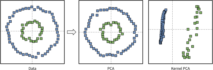
Two concentric rings, and their first two principal components (horizontal and vertical axes), computed by PCA and by kernel PCA with a Gaussian kernel. PCA only rotates the data, and no direction separates the rings. Kernel PCA separates them along its first principal component.
The following function implements kernel PCA with the Gaussian kernel, and returns the first \(k\) principal components of each point:
def kernel_pca(X, k, sigma):
    K = np.exp(-((X[:, None] - X) ** 2).sum(2) / (2 * sigma**2))  # the Gaussian kernel
    J = np.full(K.shape, 1 / len(X))  # the matrix 1_n
    Kc = K - J @ K - K @ J + J @ K @ J  # centered in the feature space
    lam, A = np.linalg.eigh(Kc)  # in the order of increasing eigenvalues
    lam, A = lam[::-1][:k], A[:, ::-1][:, :k]  # the k largest ones
    return Kc @ (A / np.sqrt(lam))  # scaled so that lam * alpha^T alpha = 1
The eigendecomposition of an \(n \times n\) matrix limits kernel PCA to datasets of moderate size, while the covariance matrix of PCA is only \(d \times d\), for \(d\) features.
t-SNE
PCA keeps the global, linear structure of the data, which is often not what one wants to see when visualizing high-dimensional data in 2D or 3D. Neighbor embedding methods instead place similar points close together, and keep the neighbors of each point.
t-SNE (t-distributed Stochastic Neighbor Embedding) turns distances into probabilities. In the input space, the similarity of point \(x_j\) to point \(x_i\) is:
\[p_{j \mid i} = \frac{\exp \left( - \| x_i - x_j \|^2 / 2 \sigma_i^2 \right)}{\sum_{k \neq i} \exp \left( - \| x_i - x_k \|^2 / 2 \sigma_i^2 \right)}\]where each \(\sigma_i\) is set so that the distribution \(p_{\cdot \mid i}\) has a given perplexity (roughly, the number of neighbors that count, typically 5 to 50), and the similarity of the pair is \(p_{ij} = (p_{j \mid i} + p_{i \mid j}) / 2n\). In the low-dimensional embedding \(y_1, ..., y_n\), the similarities follow a Student t-distribution with one degree of freedom:
\[q_{ij} = \frac{\left(1 + \| y_i - y_j \|^2 \right)^{-1}}{\sum_{k \neq l} \left( 1 + \| y_k - y_l \|^2 \right)^{-1}}\]and the embedding minimizes the Kullback-Leibler divergence \(KL(P \| Q) = \sum_{i \neq j} p_{ij} \log (p_{ij} / q_{ij})\) by gradient descent, with:
\[\frac{\partial KL}{\partial y_i} = 4 \sum_{j} (p_{ij} - q_{ij}) (y_i - y_j) \left( 1 + \| y_i - y_j \|^2 \right)^{-1}\]The heavy tails of the t-distribution let moderately distant points move far apart in the embedding, which gives well-separated clusters. Note that the sizes of the clusters and the distances between them in a t-SNE plot carry little meaning, and that the result depends on the perplexity and on the random initialization. Each iteration costs \(O(n^2)\) operations.
The following picture illustrates the iterations of t-SNE on the handwritten digits of the SOM example:
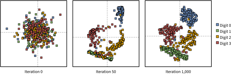
t-SNE of images of the digits 0 to 3, colored by their digit, which t-SNE does not see. The embedding starts as a small random cloud. The first iterations multiply the \(p_{ij}\) by 4 (early exaggeration), which pulls the points of each digit together, and the following ones spread the clusters apart. Each panel has its own scale.
The following function implements t-SNE. First, it finds each \(\sigma_i\) by bisection, so that \(p_{\cdot \mid i}\) has the given perplexity. Then, it runs gradient descent from a small random cloud, with the early exaggeration of the picture:
def tsne(X, perplexity=30, steps=1000, eta=100, seed=0):
    n = len(X)
    D = ((X[:, None] - X) ** 2).sum(2)
    P = np.zeros((n, n))
    for i in range(n):  # sigma_i by bisection on log(beta), with beta = 1 / 2 sigma_i^2
        d, lo, hi = np.delete(D[i], i), -50.0, 50.0
        for _ in range(60):
            b = (lo + hi) / 2
            p = np.exp(-np.exp(b) * (d - d.min()))  # d.min() avoids an underflow
            p /= p.sum()
            H = -(p * np.log2(p + 1e-300)).sum()  # the perplexity is 2^H
            lo, hi = (b, hi) if 2**H > perplexity else (lo, b)
        P[i, np.arange(n) != i] = p
    P = (P + P.T) / (2 * n)
    Y = np.random.default_rng(seed).normal(0, 1e-2, (n, 2))  # a small random cloud
    for t in range(steps):
        num = 1 / (1 + ((Y[:, None] - Y) ** 2).sum(2))  # (1 + |y_i - y_j|^2)^-1
        np.fill_diagonal(num, 0)
        Q = num / num.sum()
        M = ((4 if t < 50 else 1) * P - Q) * num  # early exaggeration of P
        G = 4 * (M.sum(1)[:, None] * Y - M @ Y)  # dKL/dy_i = 4 sum_j M_ij (y_i - y_j)
        Y -= eta * G
    return Y
UMAP follows the same idea with a graph of the nearest neighbors of each point, and is faster and keeps more of the global structure of the data. In practice, t-SNE and UMAP are used to visualize clusters, while PCA is used to compress the data or to prepare it for other methods, as it is fast and linear.
Independent Component Analysis
Independent Component Analysis (ICA) separates a signal into the independent sources that were mixed to produce it. The classic example is the cocktail party problem: several guests speak at the same time, and each microphone of the room records a different mixture of their voices. With the voices \(s(t)\) and the recordings \(x(t)\) at time \(t\), the mixing is given by:
\[x(t) = A s(t)\]where \(A\) is an unknown, invertible mixing matrix. ICA finds the unmixing matrix \(B = A^{-1}\), so that \(s(t) = B x(t)\). It assumes that the sources are statistically independent, and that at most one of them is Gaussian.
The key idea comes from the central limit theorem: a sum of independent variables is closer to a Gaussian than the variables themselves. Thus, a mixture of the sources is more Gaussian than each source, and the least Gaussian directions of the data are the sources. A simple measure of non-Gaussianity is the kurtosis, which is zero for a Gaussian, and is given for a variable \(y\) of zero mean and unit variance by:
\[\mathrm{kurt}(y) = \mathbb{E}[y^4] - 3\]ICA then runs in two steps:
- whitening: the centered data is transformed as in PCA, \(z = V x\), with \(V = \Lambda^{-1/2} F^T\), where \(\Lambda\) holds the eigenvalues and \(F\) the eigenvectors of the covariance matrix of \(x\). The whitened signals \(z\) are uncorrelated and of unit variance, and the sources are now only a rotation of them, \(s = U z\), with an orthogonal matrix \(U\). This is where ICA differs from PCA: every rotation of \(z\) is uncorrelated too, so the covariance alone cannot find \(U\), and ICA picks it with a higher-order statistic, the kurtosis;
- rotation: each row \(w^T\) of \(U\) is the unit vector that maximizes \(\vert \mathrm{kurt}(w^T z) \vert\). For \(\| w \| = 1\), the gradient of \(\mathrm{kurt}(w^T z)\) is \(4 \left( \mathbb{E}[z (w^T z)^3] - 3w \right)\), and the fixed-point iteration of FastICA moves \(w\) to this direction until it no longer changes:
The other rows are found in the same way, keeping each new \(w\) orthogonal to the rows found before. The following picture illustrates both steps:
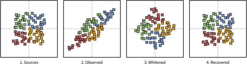
ICA of two mixed signals, with colors that mark the four quadrants of the sources. 1. The sources \(s_1\) and \(s_2\), independent and uniform. 2. The observed signals \(x = As\): the mixing turns the square into a parallelogram. 3. The whitened signals \(z = Vx\): a square again, rotated. 4. The sources recovered as \(Uz\). Inspired by: T. Yokota, Independent Component Analysis for Blind Source Separation, 2012
The following function implements ICA with FastICA. It returns the sources up to their order and signs, which ICA cannot recover:
def fast_ica(X, steps=100, seed=0):
    Xc = X - X.mean(0)  # one sample x(t) per row
    lam, F = np.linalg.eigh(np.cov(Xc, rowvar=False))
    Z = Xc @ F / np.sqrt(lam)  # the whitened signals z = V x, with V = Lambda^-1/2 F^T
    rng = np.random.default_rng(seed)
    U = np.zeros((Z.shape[1], Z.shape[1]))
    for i in range(len(U)):  # each row w of U
        w = rng.normal(size=len(U))
        for _ in range(steps):
            w = Z.T @ (Z @ w) ** 3 / len(Z) - 3 * w  # w = E[z (w^T z)^3] - 3w
            w -= U[:i].T @ (U[:i] @ w)  # orthogonal to the rows found before
            w /= np.sqrt(w @ w)
        U[i] = w
    return Z @ U.T  # the sources s = U z, up to their order and signs
Note that the kurtosis is very sensitive to outliers, as it is a fourth-order function. The negentropy is a more robust measure of non-Gaussianity.
Comparison of the Dimensionality Reduction Methods
The following table sums up the dimensionality reduction methods of this post:
| Method | Keeps | Linear | When to use it |
|---|---|---|---|
| PCA | The directions of largest variance | Yes | Compression, denoising, and a first step before other methods |
| Kernel PCA | The directions of largest variance in the feature space of a kernel | No | Non-linear structure in small to medium datasets |
| t-SNE | The neighbors of each point | No | Visualization of clusters in 2D or 3D |
| ICA | The directions of independent, non-Gaussian signals | Yes | Blind source separation, e.g. the cocktail party problem |
These methods are often combined: t-SNE is usually run on the first 30 to 50 principal components of the data, which removes noise and makes the distances cheaper to compute.