Algebra for ML Engineers
A brief summary of topics in Algebra that are relevant to ML engineers on a daily basis. Extracted from the books in the resources section. For the topics of statistics or probabilities, see the post Statistics for ML Engineers .
Properties of Matrices
- Matrices have the properties of associativity \((AB)C = A(BC)\) and distributivity \((A+B)C = AC + BC\) and \(A(B+C)=AB+AC\);
- There is no division operator defined between matrices. The equivalent is the multiplication by the inverse (when it exists) i.e. \(A/B = AB^{-1}\).
- Inverse: not every matrix \(A\) contains an inverse \(A^{-1}\). If it exists, \(A\) is called regular/invertible/non-singular. Otherwise it is called singular/non-invertible;
- \(AA^{-1} = I = A^{-1}A\), \((AB)^{-1}=B^{-1}A^{-1}\);
- two matrics \(A\) and \(B\) are inverse to each other if \(AB=I=BA\);
- Transpose: \({(A^{\intercal})^{\intercal}}=A\), \((A+B)^{\intercal}=A^{\intercal}+B^{\intercal}\), \((AB)^{\intercal}=B^{\intercal}A^{\intercal}\);
- Symmetric iff \(A=A^{\intercal}\). Thus \(A\) is square. Also, if \(A\) is symmetric and invertible then \(A^{\intercal}\) is also invertible and \(A^{\intercal}=A^{-1}\). Sum of symmetric matrices is a symmetric matrix, but product of symmetric matrices is usually not.
Systems of Linear Equations
A System of Linear Equations with equations of the type \(a_1x_1 + ...+ a_nx_n = b\) for constants \(a_1\) to \(a_n\) and \(b\) and unkownn \(x\) can be defined as \(A x=b\). The general solution of a SLE is found analytically or with Gaussian Elimination of the augmented matrix \([A \mid b]\);
- We can have none, one or infinitely many solutions to such system (when there are more unknowns than equations). When no solution exists for \(Ax=b\) we wave to resort to approximate solutions;
- The solution represents the interception of all lines (defined by diff. equations) in a geometric representation;
- Analytically:
- When \(A\) is square and invertible, the solution for \(Ax=b\) is \(x=A^{-1}b\);
- Otherwise, \(Ax = b \Leftrightarrow A^{\intercal} Ax = A^{\intercal}b \Leftrightarrow x = (A^{\intercal}A)^{−1}A^{\intercal}b\), which is also the solution to the Least Squares problem;
- \((A^{\intercal}A)^{−1}A^{\intercal}\) is also called the pseudo-inverse of \(A\), which can be computed for non-square matrices \(A\). It only requires that \(A^{\intercal}\) is positive definite, which is the case if \(A\) is full rank;
- \(\mathbb{E}[x] = (A^{\intercal}A)^{−1}A^{\intercal} \, \mathbb{E}[b] = (A^{\intercal}A)^{−1}A^{\intercal}(Ax) = x\).
- Let \(P=(A^{\intercal}A)^{−1}A^{\intercal}\).
\(\,\mathbb{Var}[x] = \mathbb{Var}[Pb] = P\, \mathbb{Var}[b] P^{\intercal} = \sigma^2 P P^{\intercal} = \sigma^2 \, (A^{\intercal}A)^{−1}A^{\intercal} \, A (A^{\intercal}A)^{-1} = \sigma^2 \, (A^{\intercal}A)^{−1}\).
We used \(\mathbb{Var}[Pb] = P \, \mathbb{Var}[b] P^{\intercal}\) (formula 375 on Matrix Cookbook), and \(A^{\intercal} \, A (A^{\intercal}A)^{-1}=I\).
- With Gaussian Elimination in \([A \mid b]\):
- The result of the forward pass of the Gaussian Elimination puts the matrix in the Row-Echelon form i.e. a staircase structure;
- A row-echelon matrix is in reduced row-echelon format if the leading entries of each row (the pivot) is 1 and the pivot is the only nonzero entry in its column;
- The result of the forward pass of the Gaussian Elimination puts the matrix in the Row-Echelon form i.e. a staircase structure;
To compute the inverse we find the matrix that satisfies \(AX=I\), so that \(X=A^{-1}\). We use Gaussian Elimination to solve the SLE \([A \mid I]\) and turn it into \([I \mid A^{-1}]\);
- Gaussian Elimination is not feasible for large matrices because of its cubic computational complexity. In practice, these are solved iteratively with e.g. the Jacobi method, Newton’s method, MCMC, etc. The main idea is:
- to solve \(Ax=b\) iteratively, we set up an iteration of the form \(x^{(k+1)} = Cx^{(k)} + d\), for a suitable \(C\) and \(d\) that minimized the residual error \(\mid x^{k+1}-x_* \mid\) in every iteration and converges to \(x_*\);
Vector Spaces
- The norm of vector \(x\) is represented by \(\| x \|\) or \(\mid x \mid\). Examples of norms: manhattan and euclidian;
- The length of a vector is \(\| x \| = \sqrt{<x,x>} = \sqrt{x^{\intercal}x}\) and the distance between two vectors is \(d(x,y) = \| x-y \| = \sqrt{ <x-y, x-y>}\);
- Cauchy-Schwarz Inequality: \(\mid <x, y> \mid \,\, \le \,\, \| x \| \, \| y \|\);
- the term vector multiplication is not well defined. Theoretically, it could be:
- an element-wise multiplication \(c_j = a_j b_j\),
- the outer product \(ab^{\intercal}\), or
- the inner product, scalar product or dot product \(<a, b> = a \cdot b = a^{\intercal}b\), which has a geometric equivalence \(a \cdot b = \vert a \vert \, \vert b \vert \, cos \, \theta\) (where \(\vert a \vert\) is the magnitude (norm) of \(a\), and \(\theta\) is the angle between \(a\) and \(b\)).
- Note: the dot product is designed specifically for the Euclidean spaces. An inner product on the other hand is a notion defined in terms of a generic vector space.
- Commutative: \(a \cdot b = b \cdot a\).
- the cross product with geometrical interpretation \(a \times b = \vert a \vert \, \vert b \vert \, sin \, \theta \, n\), that returns a vector instead of a scalar as in dot product. Not commutative: \(a \times b \neq b \times a\).
- a linear combination \(v\) of vectors \(x_1, ..., x_n\) is defined by the sum of a scaled set of vectors, ie \(v = \sum_{i=1}^k \lambda_i x_i \in V\), for constants \(\lambda_i\);
- if there is a linear combination of vectors \(x_1, ..., x_n\) such that \(\sum_{i=1}^k \lambda_i x_i=0\) with all \(\lambda_i \neq 0\), then vectors \(x\) are linearly dependent. If only the trivial solution exists with all \(\lambda_i=0\) then they are linearly independent ;
- Intuitively, a set of linearly independent vectors consists of vectors that have no redundancy, i.e., if we remove any of those vectors from the set, we will lose something in our representation;
- To find out if a set of vectors are linearly independent, write all vectors as columns of a matrix and perform the forward pass of Gaussian Elimination, ie until the row echelon form. All column vectors are linearly independent iff all columns are pivot columns;
- Otherwise, all vectors in a column without a pivot can be expressed as a linear combination of the other vectors with a pivot (as they’re the basis of that vector space);
- for a given vector space, if every vector can be expressed as a linear combination of a set of vectors \(A=\{ x_1, ..., x_n\}\), then \(A\) is the generating set of that vector space. The set of all linear combinations of \(A\) is called the span of \(A\). Moreover, \(A\) is called minimal if there exists no smaller set that spans V. Every linearly independent generating set of V is minimal and is called a basis of V;
- a basis is a minimal generating set and a maximal linearly independent set of vectors;
- the dimension of a vector space corresponds to the number of its basis vectors;
- a basis of a vector space can be found by the row-echelon form of a matrix with the spanning vectors of the space as columns. The vector defined by the columns with a pivot are a basis of U;
- the rank of a matrix is the number of linearly independent columns/rows. Thus, \(rk(A)=rk(A^{\intercal})\);
- a matrix \(A \in \mathbb{R}^{m \times n}\) is invertible iff \(rk(A)=n\);
- a SLE \(Ax=b\) can only be solved if \(rk(A) = rk (A \mid b)\);
- a matrix has full rank if its rank equals the largest possible rank for a matrix of its dimensions, otherwise it’s rank deficient;
- note: dimension of a matrix is the number of vectors in any basis for the space to be spanned. Rank of a matrix is the dimension of the column space;
Linear Mapping
A Linear Mapping (a.k.a linear transformation or map) is a function \(\phi: V \rightarrow W\) for vector spaces \(V\), \(W\), such that: \(\phi (\lambda x + \psi y) = \lambda \phi(x) + \lambda \psi(y)\), for constants \(\lambda, \psi\) and \(x, y \in V\). It can also be represented as a matrix (not only as a function).
- \(\phi\) is called injective if \(\phi(x)=\phi(y) \rightarrow x = y\); \(\,\,\) Surjective if \(\phi(V)=W\); \(\,\,\) Bijective if both;
- Surjective means that every element in \(W\) can be achieved from \(V\);
- Bijective means mapping can be undone i.e. there’s a mapping \(\psi : W \rightarrow V\) s.t. \(\psi(W)=V\);
- Special cases: Isomorphism \(\phi: V \rightarrow W\) if linear and bijective. Endomorphism \(\phi : V \rightarrow V\) if linear. Automorphism \(\phi V \rightarrow V\) if linear and bijective;
- Vector spaces \(V\) and \(W\) are isomorphic if \(dim(V) = dim(W)\). I.e. there exists a linear, bijective mapping between two vector spaces of the same dimension.
- For linear mappings \(Φ : V → W\) and \(Ψ : W → X\), the mapping \(Ψ ◦ Φ : V → X\) is also linear;
- If \(Φ : V → W\) is an isomorphism, then \(Φ^{−1} : W → V\) is an isomorphism, too.
- for \(y=Ax\), where \(x\) are a set coordinates, \(A\) is the transformation matrix of \(x\) into the new coordinates \(y\), i.e. transformation matrix can be used to map coordinates with from an ordered basis into another ordered basis;
- two matrices \(A, B \in \mathbb{R}^{m\ times n}\) are equivalent if there exist regular matrices \(S \in \mathbb{R}^{n \times n}\) and \(T \in \mathbb{R}^{m \times m}\), such that: \(B = T^{-1}A S\). I.e. the matrices can be transformed into one another by a combination of elementary row and column operations.
- two matrices \(A, B \in \mathbb{R}^{m\ times n}\) are similar if there exists a regular matrix \(S \in \mathbb{R}^{n \times n}\), such that: \(B = S^{-1}A S\). Thus, similar matrices are always equivalent, not the other way around;
- for \(\phi : V \rightarrow W\), a kernel is the set of vectors \(v \in V\) that \(\phi\) maps onto the neutral element \(0_W \in W\), ie \(\{ v \in V : \phi(v)=0_W \}\);
- the kernel space (\(ker\), or domain or null space) of a linear mapping is the solution to the SLE \(Ax=0\), ie captures all possible linear combinations of the elements in \(R^n\) that produce \(0\);
- the image (\(Im\), or codomain) of a linear mapping is the set of vectors \(w \in W\) that can be reached by \(Φ : V → W\) from any vector in \(V\);
- for a linear mapping \(Φ : V →W\), we have that \(\,\,ker(Φ) \subseteq V\) and \(Im(Φ) \subseteq W\).
- Rank-Nullity theorem: \(dim(ker(Φ)) + dim(Im(Φ)) = dim(V)\), For vector spaces \(V\), \(W\) and a linear mapping \(Φ : V →W\)
- An affine mapping / transformation is a composition of linear transformations that defines translation, scaling, rotation and shearing. Affine transformations keep the structure invariant, and preserve parallelism and dimension.
Analytic Geometry
A bilinear mapping \(\Omega : V \times V \rightarrow V\) is called symmetric if the order of the arguments doesnt matter for the final result, positive definite if \(∀x \in V \setminus {0} : Ω(x, x) > 0 , Ω(0, 0) = 0\);
A symmetric matrix \(A\) is called symmetric, positive definite or just positive definite iff it satisfies \(∀x ∈ V\setminus {0} : x^{\intercal}Ax > 0\). If only \(\ge\) holds, it is instead positive semidefinite.
- Loosely speaking, Positive-definite matrices are the matrix analogues to positive numbers. As an example: the covariance matrix is positive semidefinite.
- a positive, symmetric, definite, bilinear mapping \(\Omega : V \times V \rightarrow V\) is called an inner product on \(V\) and is typically written as \(<x,y>\). If \(A\) is p.s.d., then \(<x,y> = \hat{x}^{\intercal}A\hat{y}\) defines an inner product where \(\hat{x}, \hat{y}\) are the coordinate representations of \(x, y \in V\).
- The following holds if \(A \in \mathbb{R}^{n \times x}\) is p.s.d:
- the null space (kernel) of \(A\) is only \(0\) because \(x^{\intercal} A x \gt 0\) for all \(x \neq 0\). This implies \(A \neq 0\) if \(x \neq 0\);
- The diagonal elements elements \(a_{ii}\) of \(A\) are positive because \(a_{ii} = e^{\intercal}_i A e_i > 0\), where \(e_i\) is the \(i\)-th vector of the standard basis in \(\mathbb{R}^n\).
- in optimization, quadratic forms on positive definite matrices \(x^{\intercal}Ax\) are always positive for non-zero \(x\) and are convex.
- Important: a positive definite matrix has all positive eigenvalues, and they are in the diagonal. As the determinant equals the products of all eigenvalues, the determinant of a positive definite matrix is positive. Non-zero determinant means that p.s.d is invertible.
A metric is a function \(d:V ×V → R\) where \((x, y) → d(x, y)\) satisfies the following:
- \(d\) is positive definite, i.e., \(d(x, y) ⩾ 0\) for all \(x, y ∈ V\) and \(d(x, y) = 0 \Leftrightarrow x = y\);
- \(d\) is symmetric, i.e., \(d(x, y) = d(y, x)\) for all \(x, y ∈ V\);
- Triangle inequality: \(d(x, z) ⩽ d(x, y) + d(y, z)\) for all \(x, y, z ∈ V\);
The angle \(w\) between two vectors is computed as \(\cos w = \frac{<x,y>}{\|x\| \|y\|}\), where \(<x,y>\) is typically the dot product \(x^{\intercal}y\).
- Thus \(\cos w = \frac{<x,y>}{\sqrt{<x,x> <y,y>}} = \frac{x^{\intercal}y}{\sqrt{x^{\intercal}xy^{\intercal}y}}\);
- if \(<x,y>=0\), both vectors are orthogonal, and we write it as \(x \perp y\) (x and y are perperdicular). If \(\|x\|=\|y\|=1\) they are orthonormal;
A square matrix \(A\) is an orthogonal matrix iff its columns are orthonormal so that \(AA^{\intercal} = I = A^{\intercal}A\), which implies \(A^{-1}=A^{\intercal}\);
The inner product of two functions \(u : \mathbb{R} \rightarrow \mathbb{R}\) and \(v: \mathbb{R} \rightarrow \mathbb{R}\) is defined as \(<u,v> = \int_a^b u(x) v(x) dx\) for lower and upper limits \(a, b < \infty\);
Let \(V\) be a vector space and \(U ⊆ V\) a subspace of \(V\). A linear mapping \(π : V → U\) is called a projection if \(π^2 = π ◦ π = π\) ie \(\pi\). In the use case of matrices, \(P\) is a projection iff \(P^2 = P\).
Matrix Decompositions
determinant properties:
- \(det(AB) = det(A) det(B)\);
- \(det(A) = det(A^{\intercal})\);
- \(det(A^{-1})=\frac{1}{det(A)}\);
- for more than 2 columns or rows: \(det(A) = \sum_{k=1}^{n} (−1)^{k+j}a_{kj} det(A_{k,j})\).
- Similar matrices have the same determinant;
- a matrix \(A\) is invertible if \(det(A) \neq 0\);
- for a diagonal matrix, the determinant is computed by the product of the diagonal elements;
- the determinant is the signed volume of the parallelepiped formed by the columns of the matrix, i.e. it can also be computed as the product of the diagonal on a matrix in row-echelon form;
- Important: \(A\) is invertible iff it has full rank;
- and a square matrix \(A \in \mathbb{R}^{n \times n}\) has \(det(A) \neq 0\) iff \(rank(A)=n\).
The trace of a square matrix is the sum of its diagonal terms, or the sum of its eigenvalues;
- for a square matrix \(A \in \mathbb{R}^{n \times n}\), \(λ ∈ \mathbb{R}\) is an eigenvalue of \(A\) and \(x ∈ \mathbb{R}^n \setminus {0}\) is the corresponding eigenvector of \(A\) if \(Ax = λx\);
Eigenvalues and eigen vectors:
- to determine the eigenvalues of \(A\), solve \(Ax = \lambda x\) or equivalently solve \(det(A - \lambda I)=0\) for \(x\);
- \(p(\lambda) = det(A - \lambda I)\) is called the characteristic polynomial;
- to determine the eigenvectors \(x_i\), solve \(Ax_i=\lambda_i x_i\) for each eigenvalue \(\lambda_i\) found previously;
- eigenvectors corresponding to distinct eigenvalues are linearly independent;
- therefore, eigenvectors of a matrix with \(n\) distinct eigenvectors form a basis of \(\mathbb{R}^n\);
- a square matrix with less (linearly independent) eigenvectors than its dimension is called defective;
Two vectors are called codirected if they point in the same direction and collinear if they point in opposite directions. All vectors that are collinear to \(x\) are also eigenvectors of A;
- Non-uniqueness of eigenvectors: if \(x\) is an eigenvector of \(A\) associated with eigenvalue \(λ\), then for any \(c ∈ \mathbb{R}\setminus\{0\}\) it holds that \(cx\) is an eigenvector of \(A\) with the same eigenvalue;
- a matrix and its transpose have the same eigenvalues, but not necessarily the same eigenvectors;
- symmetric, positive definite matrices – like the p.s.d. covariance matrix – always have positive, real eigenvalues. Determinant is the product of eigenvalues, thus it is not zero. Therefore it is also invertible;
- Given a matrix \(A \in \mathbb{R}^{m \times n}\), we can always obtain a symmetric positive semidefinite matrix \(S=A^{\intercal}A\).
- If \(rk(A)=n\), then \(A^{\intercal}A\) is symmetric positive definite;
- there exists eigenvectors with real eigenvalues (spectral theorem), i.e. to check if a is positive definite, check if all eigenvalues are positive.
- Graphical intuition: the direction of the two eigenvectors correspond to the canonical basis vectors i.e., to cardinal axes. Each axis is scaled by a factor equivalent to its eigenvalue:

image source: Mathematics for Machine Learning book
Cholesky Decomposition: a symmetric, positive definite matrix \(A\) can be factorized into a product \(A = LL^{\intercal}\), where \(L\) is a lower-triangular matrix with positive diagonal elements. \(L\) is unique. This can be solved normally as a SLE. It is used e.g. to sample from Gaussian distributions and to compute determinants efficiently, as \(det(A) = det(L) det(L^⊤) = det(L)^2\).
Diagonalizable: a matrix \(A \in \mathbb{R}^{n \times n}\) is diagonalizable if it is similar to a diagonal matrix, i.e. if there is an invertible matrix \(P \in \mathbb{R}^{n \times n}\) such that \(D=P^{-1}AP\). The inverse of a diagonal matrix is the matrix replacing all diagonals by their reciprocal, i.e. replace \(a_{ii}\) by \(\frac{1}{a_{ii}}\).
- a matrix \(A \in \mathbb{R}^{n \times n}\) can be factored into \(A = PDP^{-1}\), where \(P \in \mathbb{R}^{n \times n}\) and \(D\) is a diagonal matrix whose diagonal entries are the eigenvalues of \(A\), iff the eigenvectors of \(A\) form a basis of \(\mathbb{R}^n\).
- when this eigendecomposition exists, then \(det(A) = det(PDP^{−1}) = det(P) \, det(D) \, det(P^{−1})\), and \(A^k = (PDP^{−1})^k = PD^kP^{−1}\);
- a symmetric matrix can always be diagonalized;
Singular Value Decomposition is a decomposition of the form \(A = U \Sigma V^{\intercal}\):

image source: Mathematics for Machine Learning book
- applicable to all matrices (not only square), and it always exists;
- \(\Sigma\) is the singular value matrix, a (non-square) matrix with only positive diagonal matrix with entries \(\Sigma_{ii} = \sigma_{i} \ge 0\), and zero otherwise. \(\sigma_{i}\) are the singular values. \(\Sigma\) is unique. By convention \(\sigma_{i}\) are ordered by value with largest at \(i=0\);
- \(U\) is orthogonal and its column vectors \(u_i\) are called left-singular values;
- orthogonal because \((UU^{\intercal}=U^{\intercal}U=I)\) i.e. it’s orthogonal and normal = orthonormal;
- the left-singular vectors of \(A\) are the eigenbasis (ie the eigenvectors) of \(AA^{\intercal}\);
- \(V\) is orthogonal and its column vectors \(v_i\) are called right-singular values;
- the right-singular vectors of \(A\) are eigenvectors of \(A^{\intercal}A\);
- Computing the SVD of \(A \in \mathbb{R}^{m \times n}\) is equivalent to finding two sets of orthonormal bases \(U = (u_1,... , u_m)\) and \(V = (v_1,... , v_n)\) of the codomain \(\mathbb{R}_m\) and the domain \(\mathbb{R}_n\), respectively. From these ordered bases, we construct the matrices \(U\) and \(V\);
- Comparing the eigendecomposition of an s.p.d matrix (\(S = S^⊤ = PDP^⊤\)) with the corresponding SVD (\(S = UΣV^⊤\)), they are equivalent if we set \(U = P = V\) and \(D = Σ\);
- matrix approximation/compression is achieved by reconstructing the original matrix using less singular values \(\sigma\). In practice, for a rank-\(k\) approximation: \(\hat{A(k)} = \sum_{i=1}^{k} \sigma_i u_i v_i^{\intercal} = \sum_{i=1}^k \sigma_i A_i\):
 \(\,\,\,\,\)
Left: intuition behind the SVD of a matrix \(A \in \mathbb{R}^{3 \times 2}\) as a sequential transformations. TThe SVD of a matrix can be interpreted as a decomposition of a corresponding linear mapping into three operations. Top-left to bottom-left: \(V^{\intercal}\) performs a basis change in \(\mathbb{R}^2\). Bottom-left to bottom-right: \(\Sigma\) scales and maps from \(\mathbb{R}^2\) to \(\mathbb{R}^3\). The ellipse in the bottom-right lives in \(\mathbb{R}^3\). The third dimension is orthogonal to the surface of the elliptical disk. Bottom-right to top-right: \(U\) performs a basis change within \(\mathbb{R}^3\). Right: example of application of SVD. Image sources: Mathematics for Machine Learning book and Workalemahu, Tsegaselassie, “Singular Value Decomposition in Image Noise Filtering and Reconstruction.” Thesis, Georgia State University, 2008
Eigenvalue Decomposition vs. Singular Value Decomposition:
- The SVD always exists for any matrix. The ED is only defined for square matrixes and only exists if we can find a bases of the eigenvectors in \(\mathbb{R}^n\);
- in SVD, domain and codomain can be vector spaces of different dimensions;
- the vectors of \(P\) in ED are not necessarily orthogonal. The vectors in the matrices \(U\) and \(V\) in the SVD are orthonormal, so they do represent rotations;
Vector Calculus
For \(h > 0\) the derivative of \(f\) at \(x\) is defined as the limit: \(\frac{df}{dx} = \lim_{x \rightarrow 0} \frac{f(x+h) - f(x)}{h}\). In the limit, we obtain the \(tangent\);
The Taylor series is a representation of a function \(f\) as an an infinite sum of terms that are expressed in terms of the function’s derivatives at a single point \(x_0\).
- the Taylor Polynomial of degree \(n\) of a function \(f\) at \(x_0\) is: \(T_n(x) = \sum_{k=0}^n \frac{f^{(k)}(x_0)}{k!}(x-x_0)^k\), where \(f^{(k)}\) is the \(k\)-th derivative of \(f\);
- If it is the Taylor Polinomial of infinite order i.e. \(T_{\infty}(x)\). If \(T_{\infty}(x)=f(x)\) it is called analytic;
- Relevance:
- in ML we often need to compute expectations, i.e., we need to solve integrals of the form: \(\mathbb{E}[f(x)] = \int f(x) p(x) dx\). Even for parametric \(p(x)\), this integral typically cannot be solved analytically. The Taylor series expansion of \(f(x)\) is a way to find an approximate solution \(\mathbb{E}[f(x)] \approx \mathbb{E}[T_k(x)]\).
- in Bayesian statistics, the posterior often involves computing integrals: \(p(x \mid y) = \frac{ p(y \mid x) p(x)}{p(y)}\), where \(p(y) = \int p(y \mid x) p(x) dx\). These integrals are often multidimensional in realistic problems, and are typically intractable analytically (except in a few special cases requiring the use of conjugate priors). Approximate inference must be applied.
- much of non-Bayesian statistics is based on maximum likelihood – finding the maximum of a (usually multidimensional) function, which involves knowledge of its derivatives, i.e. differentiation. Numerical methods may not be mandatory but they will be used as they are simpler (faster) – it comes down to the fact that differentiation is more tractable than integration.
- see Taylor expansions for the moments of functions of random variables for more details
The Newton’s method is a root-finding algorithm which produces successively better approximations to the roots (or zeroes) of a real-valued function. I.e. solves equations of the form \(f(x)=0\) by successive approximation. Iterations are defined as: \(x_{n+1}=x_{n}-{\frac {f(x_{n})}{f'(x_{n})}}\).
- the initial value \(x_0\) should be picked as close as possible to the zero.
- we then find the equation of the line tangent to \(y=f(x)\) at \(x=x_0\) and follow it back to the \(x\) axis at a new improved guess \(x_1\):
- the minimum of a function can be found by computing the root of the derivative ie: \(x_{n+1}=x_{n}-{\frac {f'(x_{n})}{f''(x_{n})}}\).
- The division is not defined, so we replace it by the multiplication by the inverse i.e. \(x_{n+1}=x_{n}- f'(x_{n}) \, f''(x_{n})^{-1}\).

(source: wikipedia entry for Newton’s method)
The gradient of Jacobian or \(\triangledown_x f(x)\) of function \(f : \mathbb{R}^n \rightarrow \mathbb{R}^n\) is the \(m \times n\) matrix of partial derivatives per variable \(\frac{df_i(x)}{x_j}\) for function \(i\) and variable \(j\) iterators. Useful rules in partial differentiation:
- Product: \((f(x) g(x))' = f'(x)g(x) + f(x)g'(x)\);
- Quotient: \(\left(\frac{f(x)}{g(x)}\right)' = \frac{f'(x)g(x) - f(x)g'(x)}{g(x)^2}\);
- Sum: \((f(x) + g(x))' = f'(x)+ g'(x)\);
- Chain: \((g(f(x))' = (g \circ f)'(x) = g'(f(x))f'(x) = \frac{df}{dg} \frac{dg}{dx}\);
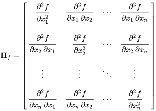
The Hessian of a function \(\triangledown^2_{x,y} f(x,y)\) is a collection of all second-order partial derivatives of all variables with respect to all other variables, defined by the symmetric matrix:
Deep Neural Networks
The output \(y\) of a \(K\)-deep DNN is computed as: \(y = (f_K ◦ f_{K−1} ◦ ... ◦ f_1)(x) = f_K(f_{K−1}( ... (f_1(x)) ... ))\)
- The chain rule allows us to describe the partial derivatives as the following:

- the orange terms are partial derivatives of a layer with respect to its inputs;
- the blue terms are partial derivatives of a layer with respect to its parameters;
Backpropagation is a special case of the automatic differentiation algorithm, a techniques to evaluate the gradient of a function by working with intermediate variables and dependencies and applying the chain rule. Example:

(source: section 5.6, Mathematics for Machine Learning)
- “Writing out the gradient in this explicit way is often impractical since it often results in a very lengthy expression for a derivative. In practice, it means that, if we are not careful, the implementation of the gradient could be significantly more expensive than computing the function, which imposes unnecessary overhead.”
-
If we use instead the automatic differentiation algorithm, we can do a forward pass efficiently by reutilizing intermediatte results, and can break the back propagation algorithm into partial derivatives that propagate backwards on the graph:

(source: adapted from example 5.14 in Mathematics for Machine Learning)
Continuous Optimization
- To check whether a stationary point is a minimum or maximum of a function, we need to take check if the second derivative is positive or negative at the stationary point. I.e. compute \(\frac{df(x)}{x^2}\), then replace \(x\) at all stationary points: If \(f′′(x)>0\), function is concave up and that point is a maximum. If \(<0\), it is concave down, and a minimum;
- Gradient Descent: an optimization method to minimize an \(f\) function iteratively. For iteration \(i\) and step-size \(\gamma\):
- \(x_{i+1} = x_t − γ((∇f)(x_i))^{\intercal}\),
- Gradient Descent with Momentum: stores the value of the update \(\Delta x_i\) at each iteration \(i\) to determine the next update as a linear combination of the current and previous gradients:
- \[x_{i+1} = x_i − γ_i((∇f)(x_i))^{\intercal} + α∆x_i\]
- where \(∆x_i = x_i − x_{i−1} = α∆x_{i−1} − γ_{i−1}((∇f)(x_{i−1}))^{\intercal}\) and \(\alpha \in [0,1]\);
- \(\alpha\) is a hyper-parameter (user defined), close to \(1\). If \(\alpha=0\), this performs regular Gradient Descent;
- Stochastic Gradient Descent: a computationally-cheaper and a noisy approximation of the gradient descent that only takes a subset of inputs at each interation;
- Constrained gradients: find \(min_x f(x)\) subject to \(g_i(x) \le 0\), for all \(i=1,...,m\);
- solved by converting from a constrained to an unconstrained problem of minimizing \(J\) where \(J(x) = f(x) + \sum_{i=1}^m \mathbb{1} (g_i(x))\);
- where \(1(z)\) is an infinite step function: \(1(z)=0\) if \(z \le 0\), and \(1(z)=\infty\) otherwise;
- and replacing this step function (difficult to optimize) by Lagrange multipliers \(\lambda\);
- the new function to minimize is now \(L(x) = f(x) + \sum_{i=1}^m \lambda_i (g_i(x)) = f(x) + \lambda^{\intercal} g(x)\)
- Lagrange duality is the method of converting an optimization problem in one set of variables x (the primal variables), into another optimization problem in a different set of variables λ (dual variables);
- further details in section 7.2 in MML book:
- solved by converting from a constrained to an unconstrained problem of minimizing \(J\) where \(J(x) = f(x) + \sum_{i=1}^m \mathbb{1} (g_i(x))\);
- Adam Optimizer (ADAptive Moment estimation): uses estimations of the first and second moments of the gradient (the curvature, exponential moving average ? ) to adapt the learning rate for each weight of the neural network;
- Curvature is not the second derivative!! This would be too expensive to compute.
- “The method computes individual adaptive learning rates for different parameters from estimates of first and second moments of the gradients.”
- in some cases Adam doesn’t converge to the optimal solution, but SGD does. According to the authors, switching to SGD in some cases show better generalizing performance than Adam alone;
- calculates the exponential moving average of gradients and square gradients. Parameters \(\beta_1\) and \(\beta_2\) are used to control the decay rates of these moving averages. Adam is a combination of two gradient descent methods, Momentum, and RMSP
- Convex sets are sets such that a straight line connecting any two elements of the set lie inside the set;
- similarly, a convex function is a function where any line segment between any two distinct points on the graph of the function lies above the graph between the two points. It’s in concave up, therefore its second derivative is non-negative on its entire domain. A strictly convex function has at most one global minimum.;
- Linear programming or linear optimization, is a method to achieve the best outcome (maximum profit or lowest cost) in a mathematical model whose requirements are represented by linear relationships, eg in the form \(f(x) = ax+b\). In algebraic notations, a linear program is defined as:
- find a vector \(x\) that maximizes/minimizes \(c^{\intercal} x\),
- subject to \(Ax \le b\) and \(x \ge 0\),
- where \(a \in \mathbb{R}^{m \times d}\) and \(b \in \mathbb{R}^m\)
- solvers: Simples, Highs, …