Statistics for ML Engineers

A brief summary of topics in statistics and probability that are relevant to ML engineers on a daily basis. Extracted from the books in the resources section. For a similar post related to the topics of Algebra, see Algebra for ML Engineers.

Basic definitions:

sample space \(Ω\) is the set of all possible outcomes of an experiment;
event space \(A\) is the space of potential results of the experiment;
probability of A, or \(P(A)\) is the degree of belief that the event \(A\) will occur, in the interval \([0,1]\);
random variable is a target space function \(X : Ω → T\) that takes an outcome/event in \(Ω\) (an outcome) and returns a particular quantity of interest \(x \in T\)
- Note: the name “random variable” creates confusion because it’s neither random nor a variable: it’s a function!
- For example, in the case of tossing two coins and counting the number of heads or tails, a random variable \(X\) maps to the three possible outcomes: \(X(hh) = 2\), \(X(ht) = 1\), \(X(th) = 1\), and \(X(tt) = 0\).
- the sum of independent random variables is the convolution: \(\int_{X+Y}(u) = \int_{-\infty}^{+\infty} f_X(u-v) \, f_Y(v) \, dv\)

Statistical distributions can be either continuous or discrete . Most parametric continuous distributions belong to the exponential family of distributions .

\(P(X=x)\) is called a probabilistic mass function (pmf) or a probability density function (pdf) for a discrete or continuous variable \(x\), respectively;
- Any discrete (continuous) domain can be a probability as long as it only has non-negative values and all values sum (integrate) to 1;
- \(P(X \le x) = = \int^x_{-\infty} p(t) dt\) is the cumulative distribution function (cdf)
  - there are CDFs which do not have a corresponding PDF;
- the probability of a subset/range of values is the sum of all probabilities of it occurring ie \(P( a \le X \le b) = \int^b_a p(t) dt\), or the equivalent sum for the discrete use case;
for discrete probabilities:
- joint probability of \(x \in X\) and \(y \in Y\) (not independent) is \(P(X=x_i, Y=y_i) = \frac{n_{ij}}{N}\), where \(n_{ij}\) can be taken as the \(ij\)-cell in the confusion matrix;

Sum rule (or marginalization property) tells that the probability of \(x\) is the sum of all joint probabilities of \(x\) and another variable \(y\):

discrete: \(p(x) = \sum_{y \in Y} p(x,y)\)
continuous: \(p(x) = \int_Y p(x,y) dy\)

Product rule relates the joint distribution and the conditions distribution, and tells that every joint distribution can be factorized into two other distributions:

\(p(x,y) = p(y \mid x) p(x) = p( x \mid y) p(y)\).

Bayes rule describes the relationship between some prior knowledge \(p(x)\) about an unobserved random variable \(x\) and some relationship \(p(y \mid x)\) between \(x\) and a second variable \(y\):

\(p(x \mid y) = \frac{ p(y \mid x) p(x)}{p(y)}\), read as: \(\text{posterior} = \frac{\text{likelihood} \times \text{prior}}{\text{evidence}}\).
derived from the product rule on both terms: \(p(y \mid x) p(y) = p(x \mid y) p(x) \Leftrightarrow p(x \mid y) = \frac{p(y \mid x) p(x)}{p(y)}\).
evidence is the marginal likelihood \(p(y) = \int p(y \mid x) p(x) dx = \mathbb{E}[ p(y \mid x)]\).
in ML the posterior \(p(\theta \mid x)\) is the quantity of interest as it tells us what we know about the parameters \(\theta\) (ie their distribution) after observing the population \(x\) (its likelihood and a known/extimated prior).

Expected Value of a function \(g\) given:

an univariate random variable \(X\) is: \(\mathbb{E}_X [g(x)] = \int_X g(x) p(x) dx\), or the equivalent averaged sum for the discrete use case.
multivariate vector as a finite set of univariate ie \(X = \left[X_1, X_2, X_D \right]\) is: \(\mathbb{E}_X [g(x)] = \left[ \mathbb{E}_{X_1} [g(x_1)], \mathbb{E}_{X_2} [g(x_2)], ..., \mathbb{E}_{X_D} [g(x_D)] \right] \in \mathbb{R}^D\).

Covariance is the expected product of their two deviations from the respective means, ue:

\(\begin{align*} \mathbb{Cov}[X,Y] & = \mathbb{E} \left[ (X- \mathbb{E}[X]) \, (Y- \mathbb{E}[Y]) \right] \\ & = \mathbb{E}\left[ XY - X\mathbb{E}[Y] - \mathbb{E}[X]Y + \mathbb{E}[X]\,\mathbb{E}[Y] \right] \\ & = \mathbb{E}[XY] - \mathbb{E}[X] \,\mathbb{E}[Y] - \mathbb{E}[X] \,\mathbb{E}[Y] + \mathbb{E}[X] \, \mathbb{E}[Y] \\ & = \mathbb{E}[XY] - \mathbb{E}[X] \,\mathbb{E}[Y] \end{align*}\).
univariate: \(\mathbb{Cov}_{X,Y}[x,y] = \mathbb{E}_{X,Y} \left[ (x-\mathbb{E}_X[x]) (y-\mathbb{E}_Y[y]) \right] = \mathbb{Cov}_{Y,X}[y,x]\)
multivariate random vars \(X\) and \(Y\) with states \(x \in \mathbb{R}^D\) and \(y \in \mathbb{R}^E\): \(\mathbb{Cov}_{X,Y}[x,y] = \mathbb{E}[xy^{\intercal}] - \mathbb{E}[x] \,\mathbb{E}[y]^{\intercal} = \mathbb{Cov}[y,y]^{\intercal} \in \mathbb{R}^{D \times E}\)

Variance:

univariate: \(\mathbb{Var}_X[x] = \mathbb{Cov}_X[x,x] = \mathbb{E}_{X} \left[ (x-\mathbb{E}_X[x])^2 \right] = \mathbb{E}_X[x^2] - \mathbb{E}_X[x]^2\)
multivariate: \(\mathbb{Var}_X[x] = \mathbb{Cov}_X[x,x] = \mathbb{E}_X[(x-\mu)(x-\mu)^{\intercal} ] = \mathbb{E}_X[xx^{\intercal}] - \mathbb{E}_X[x] \, \mathbb{E}_X[x]^{\intercal}\)
- this is a \(D \times D\) matrix also called the Covariance Matrix of the multivariate random var \(X\).
  - it is symmetric and positive semidefinite;
  - the diagonal terms are 1, i.e. no covariance between the same 2 random variables;
  - the off-diagonals are \(\mathbb{Cov}[x_i, x_j]\) for \(i,j = 1, ..., D\) and \(i \neq j\).
Law of total variance: \(\mathbb{Var}[Y] = \mathbb{E} \left [ \mathbb{Var}[Y \mid X] \right] + \mathbb{Var}\left[ \mathbb{E}[Y \mid X] \right]\)

Correlation between random variables is a measure of covariance standardized to a limited interval \([-1,1]\):

computed from the Covariance (matrix) as \(corr[x,y] = \frac{\mathbb{Cov}[x,y]}{\sqrt{\mathbb{Var}[x] \mathbb{Var}[y]}} \in [-1, 1]\)
positive correlation means \(y\) increases as \(x\) increases (1=perfect correlation). Negative means \(y\) decreases as \(x\) increases. Zero means no correlation.

Rules of transformations of Random Variables:

\(\mathbb{E}[x+y] = \mathbb{E}[x] + \mathbb{E}[y]\).
\(\mathbb{E}[x-y] = \mathbb{E}[x] - \mathbb{E}[y]\).
\(\mathbb{Var}[x+y] = \mathbb{Var}[x] + \mathbb{Var}[y] + \mathbb{Cov}[x,y] + \mathbb{Cov}[y,x]\).
\(\mathbb{Var}[x-y] = \mathbb{Var}[x] + \mathbb{Var}[y] - \mathbb{Cov}[x,y] - \mathbb{Cov}[y,x]\).
\(\mathbb{E}[Ax+b] = A \mathbb{E}[x] = A \mu\), for the affine transformation \(y = Ax + b\) of \(x\), where \(\mu\) is the mean vector.
\(\mathbb{Var}[Ax+b] = \mathbb{Var}[Ax] = A \mathbb{Var}[x] A^{\intercal} = A \Sigma A^{\intercal}\), where \(\Sigma\) is the covariance matrix.

Statistical Independence of random variables \(X\) and \(Y\) iff \(p(x,y)=p(x)p(y)\). Independence means:

\(p(y \mid x) = p(y)\).
\(p(x \mid y) = pxx)\).
\(\mathbb{E}[x,y] = \mathbb{E}[x] \, \mathbb{E}[y]\), thus
\(\mathbb{Cov}_{X,Y}[x,y] = \mathbb{E}[x,y] - \mathbb{E}[x] \, \mathbb{E}[y] = 0\), thus
\(\mathbb{Var}_{X,Y}[x+y] = \mathbb{Var}_X[x] + \mathbb{Var}_X[y]\).
important: \(\mathbb{Cov}_{X,Y}[x,y]=0\) does not hold in converse, i.e. zero covariance does not mean independence!

Conditional Independence of rvs \(X\) and \(Y\) given \(Z\) ie \(X \perp Y \mid Z\) iff \(p(x,y \mid z) = p(x \mid z) \, p(y \mid z)\) for all \(z \in Z\)

Gaussian Distribution (see the post about the Exponential Family of Distributions for more distributions):

univariate with mean \(\mu\) and variance \(\sigma^2\): \(\,\,\,p(x \mid \mu, \sigma^2 ) = \frac{1}{ \sqrt{2 \pi \sigma^2} } \,\, exp \left( - \frac{(x - \mu)^2}{2 \sigma^2} \right)\)
multivariate with mean vector \(\mu \in \mathbb{R}^D\) and covariance matrix \(\Sigma\): \(p(x \mid \mu, \Sigma ) = (2 \pi)^{-\frac{D}{2}} \mid\Sigma\mid^{-\frac{1}{2}} \exp \left( -\frac{1}{2}(x-\mu)^{\intercal} \Sigma^{-1}(x-\mu) \right)\)
marginals and conditional of multivariate Gaussians are also Gaussians:
- joint distribution of a bivariate Gaussian distribution made of two Gaussian random variables \(X\) and \(Y\): \(p(x,y) = \mathcal{N} \left( \begin{bmatrix} \mu_x \\ \mu_y \end{bmatrix}, \begin{bmatrix} \Sigma_{xx} & \Sigma_{xy} \\ \Sigma_{yx} & \Sigma_{yy} \end{bmatrix} \right)\).
- the conditional is also Gaussian: \(p(x \mid y) = \mathcal{N} ( \mu_{x \mid y} , \Sigma_{x \mid y})\).
- the marginal is also Gaussian: \(p(x) = \int p(x,y) dy = \mathcal{N} ( x \mid \mu_x, \Sigma_{xx})\).
A bivariate Gaussian. Green: joint density p(x,y). Blue: marginal density p(x). Red: marginal density p(y). The conditional disribution is a slice accross the X or Y dimension and is also a Gaussian. Source: wikipedia page for Multivariate normal distribution
the product of two gaussians pdfs \(\mathcal{N} (x \mid a, A) \, \mathcal{N}(x \mid b, B)\) is a Gaussian scaled by a \(c \in \mathbb{R}\).
if \(X,Y\) are independent univariate Gaussian random variables:
- \(p(x,y)=p(x) p(y)\), and
- \(p(x+y) = \mathcal{N}(\mu_x + \mu_y, \Sigma_x + \Sigma_y)\).
  - weighted sum \(p(ax + by) = \mathcal{N}(a\mu_x + b\mu_y, a^2 \Sigma_x + b^2 \Sigma_y)\).
any linear/affine transformation of a Gaussian random variable is also Guassian. Take \(y=Ax\) being the transformed version of \(x\):
- \(\mathbb{E}[y] = \mathbb{E}[Ax] = A \mathbb{E}[x] = A\mu\), and
- \(\mathbb{Var}[y] = \mathbb{Var}[Ax] = A \mathbb{Var}[x]A^T = A \Sigma A^{\intercal}\), thus
- \(p(y) = \mathcal{N}(y \mid A\mu, A \Sigma A^{\intercal})\).
sum of uniform gaussians squares \(Z_i \sim \mathcal{N}(0,1)\)is a Chi-Square distribution with \(n\) degrees of freedom: \(Z_1^2 + Z_2^2 + ... + Z_n^2 \sim X_n^2\).

Conjugacy

If the posterior distribution \(p(\theta \mid x)\) is in the same probability distribution family (not only same distribution) as the prior \(p(\theta )\):
- the prior and posterior are then called conjugate distributions, and
- the prior is called a conjugate prior for the likelihood function \(p(x\mid \theta )\).
A conjugate prior is an algebraic convenience, giving a closed-form expression for the posterior; otherwise, numerical integration may be necessary.
Every member of the exponential family has a conjugate prior.

Exponential Family is the family of distributions that can be expressed in the form \(p(x \mid \theta) = h(x) \exp \left(\eta(\theta)^{\intercal} ϕ(x) -A(\theta)\right)\)

\(θ\) are the the natural parameters of the family
\(A(θ)\) is the log-partition function, a normalization constant that ensures that the distribution sums up or integrates to one.
\(ϕ(x)\) is a sufficient statistic of the distribution
- we can capture information about data (population) in \(ϕ(x)\).
- sufficient statistics carry all the information needed to make inference about the population, that is, they are the statistics that are sufficient to represent the distribution:
- Fischer-Neyman theorem: Let \(X\) have probability density function \(p(x \mid θ)\). Then the statistics \(ϕ(x)\) are sufficient for \(θ\) if and only if \(p(x \mid θ)\) can be written in the form \(p(x \mid \theta) = h(x) g_{\theta}(ϕ(x))\), where \(h(x)\) is a distribution independent of \(θ\) and \(g_θ\) captures all the dependence on \(θ\) via sufficient statistics \(ϕ(x)\).
- Note that the form of the exponential family is essentially a particular expression of \(g_θ(ϕ(x))\) in the Fisher-Neyman theorem.
\(\eta\) is the natural parameter,
for optimization purposes, we use \(p (x \mid \theta) \propto \exp (\theta^{\intercal} ϕ(x))\).
Why use exponential family:
- they have finite-dimensional sufficient statistics;
- conjugate distributions are easy to write down, and the conjugate distributions also come from an exponential family;
- Maximum Likelihood Estimation behaves nicely because empirical estimates of sufficient statistics are optimal estimates of the population values of sufficient statistics (recall the mean and covariance of a Gaussian);
- From an optimization perspective, the log-likelihood function is concave, allowing for efficient optimization approaches to be applied;
Alternative notation in natural form: \(p(x \mid \eta) = h(x) \exp \left(\eta^T T(x) -A(\eta)\right)\).

Moment Generation Function is an alternative formulation of a pdf \(f(x)\):

\(M(t) = \mathbb{E} \left[ e^{eX} \right] = \sum_{x \in S} e^{tX}\, f(x)\).
if distributions are independent: \(M_{X+Y}(t) = M_X(t) * M_Y(Y)\).
can be used to show that e.g. sum of gaussians is a gaussian.

Central Limit Theorem: Let \(Y_n\) be independent random variables (of any form) with \(\mathbb{E}[Y_k]=\mu\) for all \(k\). Then \(\frac{1}{n} (Y_1 + ... + Y_n) \rightarrow \mu\).

Law of Large Numbers: Let \(\{ Y_n \}\) be a sequence of iid random variables (of any form) with mean \(\mu\) and variance \(\sigma^2\). Then \(\sqrt{n} \left( \frac{1}{n} \sum_{i=1}^N (Y_i - \mu) \right) \rightarrow \mathcal{N}(0, \sigma^2)\).

Inequality rules:

Jensen’s inequality: \(\phi (\mathbb{E}[X]) \le \mathbb{E}[ \phi(X)]\) , where \(\phi\) is a convex function.
Markov’s inequality: \(p(X \ge \epsilon) \le \frac{\mathbb{E}[X]}{\epsilon}\), where \(\epsilon \gt 0\).
Chebyshev’s inequality: \(p \left( \mid X - \mathbb{E}[X] \mid \ge \epsilon \right) \le \frac{\mathbb{Var}[X]}{\epsilon^2}\).
Chauchy-Schwarz inequality: \(\mathbb{Var}[A] \, \mathbb{Var}[B] \ge \mathbb{Cov}^2[A,B]\).
ELBO inequality: \(\ln p_{\theta }(x)\geq \mathbb {\mathbb {E} } _{z\sim q_{\phi }}\left[\ln {\frac {p_{\theta }(x,z)}{q_{\phi }(z)}}\right].\)
- the left-hand side is the evidence for \(x\), and the right-hand side is the evidence lower bound (ELBO) for \(x\).

Kullback–Leibler / KL divergence: \(KL ( q \| p ) = \int_\mathbb{R} p(x) \log \frac{p(x)}{q(x)} dx\)

from Jensen’s inequality we get: \(KL ( q \| p ) = \mathbb{E} \left[ - \log \frac{q(X)}{p(X)} \right] \ge -\log \mathbb{E} \left[ \frac{q(X)}{p(X)} \right] =0\).
KL divergence is not a metric because it’s not symmetric: \(KL ( q \| p ) \neq KL ( p \| q )\).
\(p=q \Leftrightarrow KL ( q \| p ) = 0\).

Testing:

quantile is the inverse of the CDF. It tells at which point the cdf (or the integral of the pdf) equals a given value \(\alpha \in [0,1]\).
p-value (or observed significance level) is the smallest value of \(α\) for which the null hypothesis would be rejected at level \(α\).
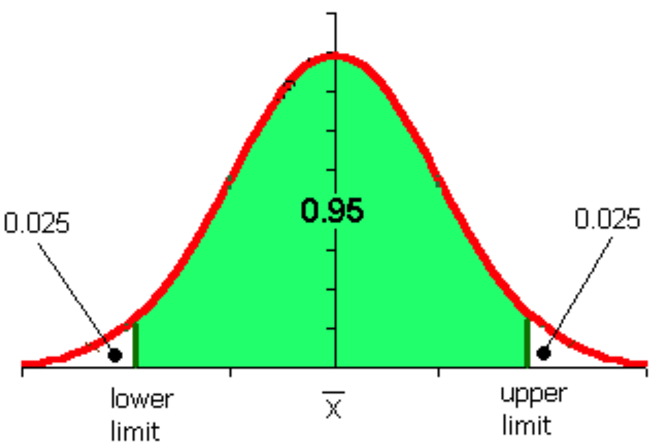
the confidence interval refers to the probability that a population parameter will fall between a set of values for a certain proportion of times. Example, for a \(95%\) confidence level:

Entropy measures the average level of surprise or uncertainty inherent to the channel:

\(\mathrm {H} (X) = -\int_{x} p(x)\log p(x)=\mathbb {E} [-\log p(x)] dx\).
Conditional Entropy: \(H( Y \mid X) = - \int_x f(x) \int_y f(y \mid x) \log f(y \mid x) \,dy\,dx\).
Joint Entropy: \(H(X, Y) = - \int_{xy} f(x,y) \log f(x,y x) \,dx\,dy\).
Entropy Chain Rule: \(H(X,Y) = H(X) + H(Y \mid X) = H(Y) + H(X \mid Y)\).

Mutual Information measures the reduction in uncertainty for one variable given a known value of the other variable:

\(I(X,Y)= \int_{x,y} p(x,y) \log \frac{p (x,y)}{p(x) \, p(y)} dx\,dy = \mathbb{E} \left[ D_{KL} \left( p(x \mid y) \,\|\, p(x) \right) \right]\).
\(I(X,Y)= H(Y) - H(Y \mid X) = H(X) - H(X \mid Y)\).

Arrangements of \(k\) items out of a set of size \(n\):

Arrangement is the arrangement of some items in which order matter: \(^nA_k=n^k\) with replacement or \(k!\) without.
Permutation is the arrangements of all items in which order matters: \(^nP_k=\frac{n!}{(n-k)!}\).
Combination is the arrangement of some items in which order doesn’t matter: \(\binom nk = \, ^nC_k = \frac{1}{k!} ^nP_k = \frac{n!}{k!(n-k)!}\).

Sets

the union of two subsets is written as \(F_1 \cup F_2 = \{ ω ∈ Ω : ω ∈ F1 \text{ or } ω ∈ F2 \}\);
the intersection is \(F1 ∩ F2 = \{ ω ∈ Ω : ω ∈ F1 \text{ and } ω ∈ F2 \}\);
two events F1 and F2 are disjoint if they have no elements in common, or \(F_1 ∩ F_2 = ∅\);
the complement of \(F\) is written as \(F^C\) and contains all elements of \(\Omega\) which are not in \(F\) ie \(F^c = \{ ω ∈ Ω : ω \not\in F \}\).
- From this we write \(F ∪ F^c = Ω\);
a partition \(\{ F_n \}\) for \(n \ge 1\) is a collection of events such that \(F_i ∩ F_j = ∅\) for all \(i \neq j\) and \(\cup_{n≥1} F_n = Ω\);
the difference between \(F_1 and F_2\) is defined as \(F1 \backslash F2 = F1 ∩ F_2^C\);
the following properties hold:
- associativity: \((F1 ∪ F2) ∪ F3 = F1 ∪ (F2 ∪ F3) = F1 ∪ F2 ∪ F3\)
- associativity: \((F1 ∩ F2) ∩ F3 = F1 ∩ (F2 ∩ F3) = F1 ∩ F2 ∩ F3\)
- distributivity: \(F1 ∩ (F2 ∪ F3) = (F1 ∩ F2) ∪ (F1 ∩ F3)\)
- distributivity: \(F1 ∪ (F2 ∩ F3) = (F1 ∪ F2) ∩ (F1 ∪ F3)\)
- De Morgan’s Laws: \((F1 ∪ F2)^c = F^c_1 ∩ F^c_2\) and \((F1 ∩ F2)^c = F^c_1 ∪ F^c_2\)

Using the previous axioms we can show that:

We can show that \(Pr(F1 ∪ F2) = Pr(F1) − Pr(F1 ∩ F2) + Pr(F2)\);
\(Pr(F1 ∩ F2) ≤ min\{Pr(F1), Pr(F2)\}\);
\(F ∪ F^c = Ω\), \(1 = Pr(Ω) = Pr(F) + Pr(F^c)\), thus \(Pr(F^c) = 1 − Pr(F)\)

Causal Inference: a Direct Aclyclic Graph is a probabilistic model for which a graph expresses the conditional dependence structure between random variables.

the model represents a factorization of the joint probability of all random variables: \(P(X_1,\ldots ,X_n) =\prod_{i=1}^{n} p \left( X_i \mid p(X_i) \right)\).
Example: \(p(A,B,C,D) = P(A)\cdot p(B \mid A) \cdot p( C \mid A) \cdot p ( D \mid A,C )\):

Source: wikipedia entry for Graphical model

Extra: Non-parametric statistics (Smoothing): we use a Kernel Density Estimator to convert a discrete distribution into a continuous distribution. Formulation: given a cumulative distribution function, discrete, formulated by \(n\) steps \(Y_1, ..., T_n\) as:

\[\hat{F}_n (y) = \frac{1}{n} \sum_{i=1}^{n} I(Y_i \le y)\]

the kernel density estimator \(\hat{f}\) is the random density function:

\[\hat{f}(x) \, = \, \frac{1}{nh} \sum_{i=1}^n K \left( \frac{x-Y_i}{h} \right)\]

where \(K\) is the kernel - a non-negative function - and \(h \gt 0\) is a the smoothing parameter (bandwidth).

\(h\) regulates bias-variance trade-off;
large \(h\) vs small \(h\) dictates flat vs wiggly estimator;
an example of \(K\) is the standard normal CDF.

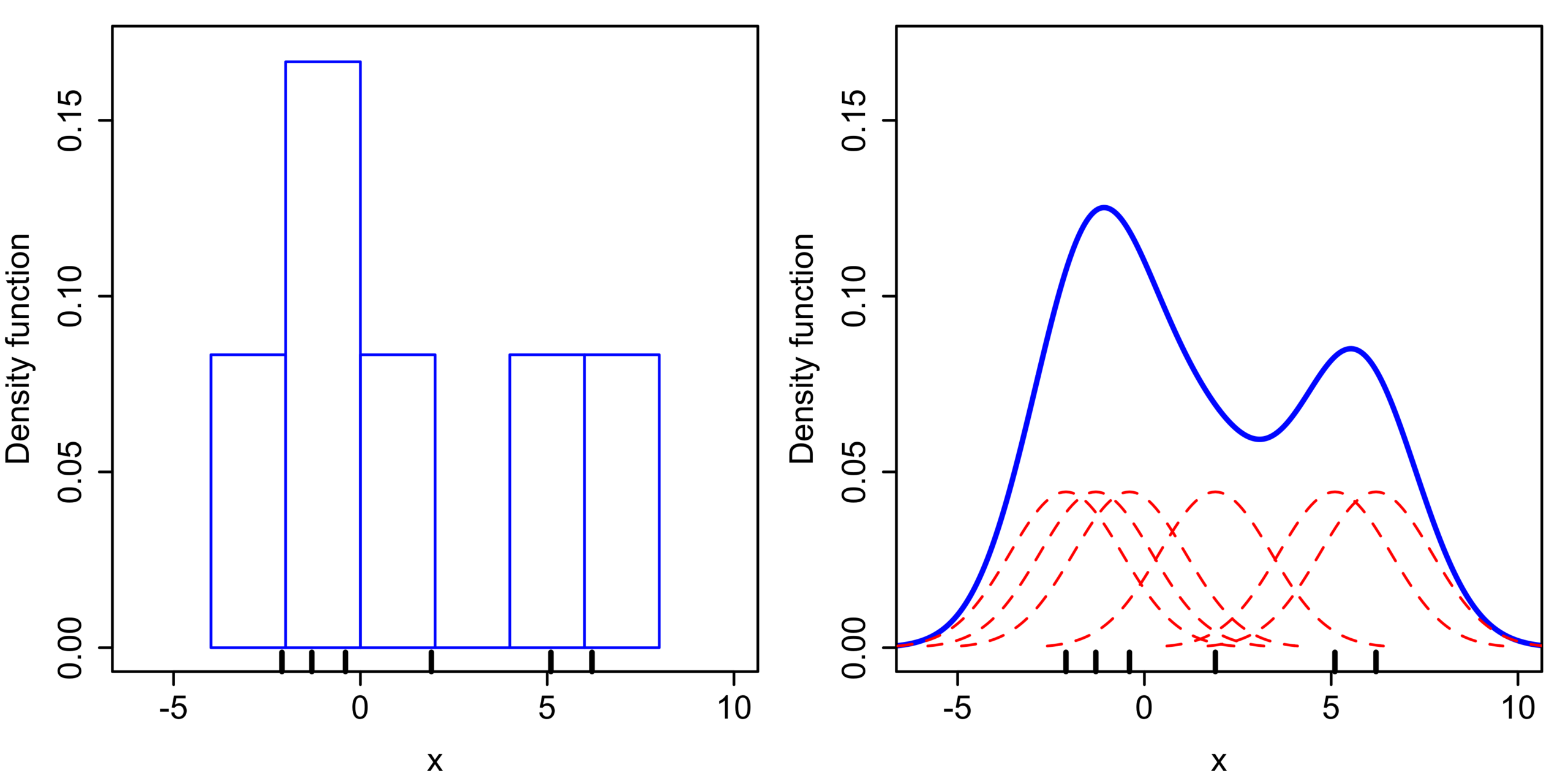
Source: wikipedia entry for Kernel density estimation

The following table summarizes the method used for each use case:

Distribution / function \(g\)	parametric \(g(x_i^{\intercal}) = x_i^{\intercal} \beta\)	non-parametric \(g\)
Gaussian	Linear Regression	Smoothing (KDE)
Exponential Family	Generalized Linear Models	Generative Additive Models