Bayesian Linear Regression, Maximum Likelihood and Maximum-A-Priori
Bayesian methods allows us to perform modelling of an input to an output by providing a measure of uncertainty or “how sure we are”, based on the seen data. Unlike most frequentist methods commonly used, where the outpt of the method is a set of best fit parameters, the output of a Bayesian regression is a probability distribution of each model parameter, called the posterior distribution.
For the sake of comparison, take the example of a simple linear regression \(y = mx + b\). On the frequentist approach, one tries to find the constant that define the slope \(m\) and bias \(b\) values, with \(m \in \mathbb{R}\) and \(b \in \mathbb{R}\). On the other hand, the Bayesian approach would also compute \(y = mx + b\), however, \(b\) and \(m\) are not assumed to be constant values but drawn from probability distributions instead. The parameters of those probabilities define the values to be learnt (or tuned) during training. A common approach is to assume as prior knowledge that \(m\) and \(b\) are independent and normally distributed — i.e. \(b \thicksim \mathcal{N}(\mu_{b}, \sigma^2_{b})\) and \(w \thicksim \mathcal{N}(\mu_{w}, \sigma^2_{w})\) — and the parameters to be learnt would then be all \(\mu\) and \(\sigma\). Additionally, on a Bayesian approach we can also add the model of the noise (inverse of the precision) constant \(\varepsilon\) that models how noisy our data may be, by computing \(y = mx + b + \varepsilon\) instead, with \(\varepsilon \thicksim \mathcal{N}(0, \sigma^2_{\varepsilon})\).
Apart from the uncertainty quantification, another benefit of Bayesian is the possibility of online learning, i.e. a continuous update of the trained model (from previously-seen data) by looking at only the new data. This is a handy feature for e.g. datasets that are purged periodically.
Refresher: Normal distribution
A probability distribution is a mathematical function that provides the probabilities of occurrence of different possible outcomes in an experiment. In the following post, we methods will be solely based on the Normal distribution defined for an input \(x\) by:
- \(p(x \mid \mu, \sigma ) = \frac{1}{ \sqrt{2 \pi \sigma^2} } \,\, exp \left( - \frac{(x - \mu)^2}{2 \sigma^2} \right)\) for a distribution with mean \(\mu\) and standard deviation \(\sigma\) on an univariate notation, or
- \(p(x \mid \mu, \Sigma ) = \left(\frac{1}{2 \pi}\right)^{-D/2} \,\, det(\Sigma)^{-1/2} exp \left( - \frac{1}{2}(x - \mu)^T \Sigma^{-1} (x-\mu) \right)\) with mean vector \(\mu\) and covariance matrix \(\Sigma\) on its multivariate (matrix) notation
Bayes Theorem
From the field of probability, the product rule tells us that \(p(A, B) = p(A) p(B\mid A)\). By symmetry we have that \(p(B,A) = p(B) p(A\mid B)\). By equating both right hand sides of the equations and re-arranging the terms we obtain the Bayes Theorem:
\begin{equation} \text{posterior} = \frac{\text{likelihood}\, \times \, \text{prior}}{\text{evidence}} = p(A\mid B) = \frac{p(B\mid A) p(A)}{p(B)}\end{equation}
In Machine Learning, we are mostly interested in how the parameters of the model \(\theta\) relate to the data \(X\):
\[p(\theta \mid X) = \frac{p(X\mid \theta) p(\theta)}{p(X)} \propto p(X \mid \theta) p(\theta) \label{eq_prior_AB}\],where evidence is \(p(X) = \int p(X \mid \theta) p(\theta) d\theta = \mathbb{E}_{\theta}[ p(X \mid \theta) ]\)
The idea behing Bayes Theorem in ML is to invert the relationship between the parameters \(θ\) and the data \(X\) to obtain the posterior;
An important theoream called the Bernstein-von Mises Theorem states that:
- for a sufficiently large sample size, the posterior distribution becomes independent of the prior (as long as the prior is neither 0 or 1)
- ie for a sufficiently large dataset, the prior just doesnt matter much anymore as the current data has enough information;
- if we let the datapoints go to infitiny, the posterior distribution will go to normal distribution, where the mean will be the maximum likelihood estimator;
- this is a restatement of the central limit theorem, where the posterior distribution becomes the likelihood function;
- ie the effect of the prior decreases as the data increases;
- we typically want to maximize the posterior, so we can drop the evidence term (as it’s independent of \(\theta\)) and compute only the maximum of the term \(p(X \mid \theta) p(\theta)\).
There are two main optimization problems that we discuss in Bayesian methods: Maximum Likelihood Estimator (MLE) and Maximum-a-Posteriori (MAP).
Maximum Likelihood Estimator (MLE)
(In case the following reductions cause some confusion, check the appendix at the bottom of the page for the rules used, or The Matrix Cookbook for a more detailed overview of matrix operations.)
When we try to find how likely is for an output \(y\) to belong to a model defined by data \(X\), weights \(w\) and model parameters \(\sigma\) (if any), or maximize the likelihood \(p(y\mid w, X, \sigma^2)\), we perform a Maximum Likelihood Estimator (MLE). Maximizing the likelihood means maximizing the probability that models the training data, given the model parameters, as:
\[w_{MLE} = argmax_w \,\, p(y \mid w, X)\]Let us interpret what the probability density \(p(x \mid θ)\) is modeling for a fixed value of θ. It is a distribution that models the uncertainty of the data for a given parameter setting. In a complementary view, if we consider the data to be fixed (because it has been observed), and we vary the parameters θ, what does the MLE tell us? It tells us how likely a particular setting of θ is for the observations x. Based on this second view, the maximum likelihood estimator gives us the most likely parameter θ for the set of data. (MML book, section 8.3.1).
When the distribution of the prior and posterior are computationally tractable, the optimization of the parameters that define the distribution can be performed using the coordinate ascent method, an iterative method that was covered in other post. In practice we perform and iterative partial derivatives of the prior/posterior for the model parameters (e.g. mean \(\mu\) and standard deviation \(\sigma\) in a Gaussian environment) and move our weight estimation towards the direction of lowest loss.
To simplify the computation, we perform the log-trick and place the term to optimize into a log function. We can do this because \(log\) is a monotonically-increasing function, thus applying it to any function won’t change the input values where the minimum or maximum of the solution (ie where gradient is zero). Moreover, since Gaussian distribution is represented by a product of exponentials, by applying the \(log\) function we bring the power term out of the exponential, making its computation simpler and faster. In practice, we apply the log-trick to the function we want to minimize and get:
\[\begin{align*} -\log \,\, p(y \mid w, X) & = -log \prod_{n=1}^N p(y_n \mid w_n, X_n) \\ & = - \sum_{n=1}^N log \,\, p(y_n \mid w_n, X_n)\\ \end{align*}\]I.e. we turn a log of products into a sum of logs. In the linear regression model, the likelihood is Gaussian, due to the Gaussian noise term \(\varepsilon \thicksim \mathcal{N}(0, \sigma^2_{\varepsilon})\). Therefore:
\[\begin{align*} log \,\, p(y \mid w, X, \sigma^2) & = \log \left( \frac{1}{ \sqrt{2 \pi \sigma^2} } \,\, exp \left( - \frac{(y_n - x_n^Tw)^2}{2 \sigma^2} \right) \right)\\ & = - \frac{1}{2 \sigma^2} (y_n - x^T_n w)^2 + const \\ \end{align*} \label{eq_lr_likelihood}\]where \(const\) includes all terms independent of \(w\). Using the negative of the previous log-likelihood, and ignoring the constants whose derivative is zero, we get the following loss function:
\[\begin{align*} L(w) & = \frac{1}{2 \sigma^2} \sum_{n=1}^N (y_n - Xw)^2 \\ & = \frac{1}{2 \sigma^2} (y - Xw)^T (y-Xw) \\ & = \frac{1}{2 \sigma^2} \| y-Xw \|^2 \\ \end{align*}\]The second trick here is that the previous equation is quadratic in \(w\). Thus we have an unique global solution for minimizing the previous log-likelihood and compute the point of minimum loss as:
\[\begin{align*} & \frac{dL}{dw} = 0 \\ \Leftrightarrow & 0 = \frac{d}{dw} \left( \frac{1}{2 \sigma^2} (y-Xw)^T(t-Xw) \right) \\ \Leftrightarrow & 0 = \frac{1}{2 \sigma^2} \frac{d}{dw} \left( y^Ty - 2y^TXw + w^TX^TXw \right) \\ \Leftrightarrow & 0 = \frac{1}{2 \sigma^2} \left( -2y^TX + 2w^TX^TX \right) \\ \Leftrightarrow & y^TX = w^TX^TX \\ \Leftrightarrow & w^T = y^TX (X^TX)^{-1} \\ \Leftrightarrow & w_{MLE} = (X^TX)^{-1}X^Ty \\ \end{align*}\]Note that this solution is independent of the noise variance \(\sigma^2\), and is the same as minimizing the Least Squares Problem, as we showed in a previous post, with the same closed-form solution \(w = (X^TX)^{-1} X^Ty\). In practice, minimizing the Least Squares problem is equivalent to determining the most likely \(w\) under the assumption that \(y\) contains gaussian noise i.e. \(y = wx + b + \varepsilon\), with \(\varepsilon \thicksim \mathcal{N}(0, \sigma^2)\).
Adding regularization
Regularizers can be added normally as in the non-Bayesian regression and may have as well an analytical solution. As an example, if we want ot add an \(L_2\)/Ridge regularizer:
\[\begin{align*} & 0 = \frac{d}{dw} \left( L - \frac{\alpha}{2} w^Tw \right)\\ \Leftrightarrow & 0 = \frac{d}{dw} \left( - \frac{D}{2} log ( 2 \pi \sigma^2) - \frac{1}{2 \sigma^2} (y-Xw)^T(y-Xw) - \frac{\alpha}{2} w^Tw \right)\\ \Leftrightarrow & w_{MLE\_reg} = (X^TX + \lambda I )^{-1} X^Ty\\ \end{align*}\]where \(\lambda = \alpha \sigma^2\), therefore the solution is now noise-dependent, contrarily to the previous use case. Note that we picked the regularizer constant \(\alpha/2\) on the first step to simplify the maths and cancel out the 2 when doing the derivative of the \(w^Tw\).
Estimating noise variance
So far we assumed the noise \(\sigma^2\) is known. However, we can use the same Maximum Likelihood principle to obtain the estimator \(\sigma^2_{MLE}\) for the noise:
\[\begin{align*} log \,\, p(y \mid X, w, \sigma^2) = & \sum_{n=1}^N log \,\, \mathcal{N} (y_n \mid X_nw, \sigma^2) \\ = & \sum_{n=1}^N \left( -\frac{1}{2} log(2\pi) -\frac{1}{2} log(\sigma^2) -\frac{1}{2 \sigma^2}(y_n-X_nw)^2 \right)\\ = & -\frac{N}{2} log \sigma^2 -\frac{1}{2 \sigma^2} \sum_{n=1}^N (y_n - X_nw)^2 + const\\ \end{align*}\]The partial derivative of the loss with respect to \(\sigma^2\) and the MLE-estimation of \(\sigma^2\) is then:
\[\begin{align*} & \frac{d \,\, log \,\, p(y \mid X, w, \sigma^2)}{d \sigma^2} = -\frac{N}{2 \sigma^2} + \frac{1}{2 \sigma^4} \sum_{n=1}^N (y_n - X_nw)^2 = 0\\ \Leftrightarrow & \frac{N}{2 \sigma^2} = \frac{1}{2 \sigma^4} \sum_{n=1}^N (y_n - X_nw)^2 \\ \Leftrightarrow & \sigma^2_{MLE} = \frac{1}{N} \sum_{n=1}^N (y_n - X_nw)^2 \\ \end{align*}\]i.e. \(\sigma^2\) is the mean of the squared distance between observations and noise-free values.
Maximum-a-Posteriori (MAP)
Maximum likelihood without regularizer is prone to overfitting (details in section 9.2.2 of the Mathematics for Machine Learning book). In the occurrence of overfitting, we run into very large parameter values. To mitigate the effect of huge values, we can place the prior on the parameter space, and seek now the parameters to estimate the posterior distribution.
If we have prior knowledge about the distribution of the parameters, we can multiply an additional term to the likelihood. This additional term is a prior probability distribution on parameters. For a given prior, after observing some data \(x\), how should we update the distribution of the parameters? In other words, how should we represent the fact that we have more specific knowledge of the parameters after observing data \(x\)?
This is called the Maximum-a-Posteriori estimation (MAP), and is obtained by applying the Bayes Theorem.
The problem in hand is to find the parameters of the distribution that best represent the data. Adapting the equation \ref{eq_prior_AB} of the prior to the problem of regression, we aim at computing:
\[p(w\mid X, y) = \frac{p(y\mid X, w) p(w)}{p(y \mid X)} \propto p(y\mid X, w) p(w) \label{posterior_w}\]The computation steps are similar to log-trick applied to the MLE use case. The log-posterior is then:
\[log \,\, p(w\mid X, y) = log \,\, p(y \mid X, w) + log \,\, p(w) + const\]In practice, this is the sum of the log-likelihood \(log \,\, p(y \mid X, w)\) and the log-prior \(log \,\, p(w)\), so the MAP estimation is a compromise between the prior and the likelihood. An alternative view is the idea of regularization, which introduces an additional term that biases the resulting parameters to be close to the original (MML book section 8.3.2). Similarly to the MLE, we compute the derivative of the negative log-posterior with respect to \(w\) as:
\[\begin{align*} & - \frac{d \,\, log \,\, p( w \mid X,y)}{dw} \\ = & \frac{d \,\, log \,\, p( y \mid X,w)}{dw} - \frac{d \,\, log \,\, p(w)}{dw} \\ = & \frac{d}{dw} \left( \frac{1}{2 \sigma^2}(y-Xw)^T(y-Xw) \right) + \frac{d}{dw} \left( \frac{1}{2b^2}w^Tw \right) & \text{(Linear Reg. likelihood (eq \ref{eq_lr_likelihood}), and prior } \mathcal{N}(0, b^2 I) \text{)}\\ = & \frac{1}{\sigma^2}(w^TX^TX-y^TX) + \frac{1}{b^2}w^T & \text{(First-order derivative, rule 3)}\\ \end{align*} \label{eq_prior_w}\]Computing the minimum value:
\[\begin{align*} & \frac{1}{\sigma^2}(w^TX^TX-y^TX) + \frac{1}{b^2}w^T = 0 \\ \Leftrightarrow & w^T \left( \frac{1}{\sigma^2}X^TX + \frac{1}{b^2}I \right) - \frac{1}{\sigma^2}y^TX = 0\\ \Leftrightarrow & w^T \left( X^TX + \frac{\sigma^2}{b^2}I \right) = y^TX \\ \Leftrightarrow & w^T = y^TX \left( X^TX + \frac{\sigma^2}{b^2}I \right)^{-1} \\ \Leftrightarrow & w^T_{MAP} = \left( X^TX + \frac{\sigma^2}{b^2}I \right)^{-1} X^Ty\\ \end{align*}\]Now we see that the only difference between the weights estimated using MAp(\(w_{MAP}\)) and using MLE (\(w_{MLE}\)) is the additional term \(\frac{\sigma^2}{b^2}I\) in the inverse matrix, acting as a regularizer.
Closed-form solution for Bayesian Linear Regression
Instead of computing a point estimate via MLE or MAP, a special case of Bayesian optimization is the linear regression with normal priors and posterior. In this case, the posterior has an analytical solution. This approach is utilized very commonly, mainly since the result is not an estimation, and computing the analytical solution for the posteriors is extremelly fast to compute even for very large datasets and dimensionality.
In brief, bayesian linear regression is a type of conditional modeling in which the mean of one variable is described by a linear combination of other variables, with the goal of obtaining the posterior probability of the regression coefficients (as well as other parameters describing the distribution of the regressand) and ultimately allowing the out-of-sample prediction of the regressand (often labelled {\displaystyle y}y) conditional on observed values of the regressors (source: wikipedia page for Bayesian Linear Regression). I.e. Bayesian linear regression pushes the idea of the parameter prior a step further and does not even attempt to compute a point estimate of the parameters, but instead the full posterior distribution over the parameters is taken into account when making predictions. This means we do not fit any parameters, but we compute a mean over all plausible parameters settings (according to the posterior).
We assume all our weights are drawn from a gaussian distribution and can be independent (if covariance matrix is diagonal) or not (otherwise). In practice, we start with the prior \(p(w) \thicksim \mathcal{N}(m_0, S_0)\), with mean vector \(m_0\), and (positive semi-definite) covariance matrix \(S_0\) (following the variable notation found on Chris Bishop’s PRML book).
We have then the following prior in multivariate notation:
\[p(w \mid m_0, S_0 ) = (2 \pi)^{-\frac{D}{2}} \,\, det(S_0)^{- \frac{1}{2}} \,\, exp \left( - \frac{1}{2}(w - m_0)^T S_0^{-1} (y-m_0) \right)\]And the likelihood:
\[p(y \mid X, w) = \frac{1}{(2 \pi \sigma^2)^{D/2}} exp \left( -\frac{1}{2 \sigma^2} (y-Xw)^T(y-Xw) \right)\]Going back to Equation \ref{posterior_w} and replacing the terms, we have:
\[\begin{align*} p(w \mid X, y) & = \frac{p(y\mid X, w) p(w)}{p(y \mid X )} \\ & \propto p(y\mid X, w) p(w) & \text{(dropped constant term in division)}\\ & \propto exp \left( -\frac{1}{2 \sigma^2} (y-Xw)^T(y-Xw) - \frac{1}{2}(w-m_0)^TS_0^{-1}(w-m_0) \right) & \text{(dropped constant in multiplication)}\\ & = exp \left( -\frac{1}{2} \left( \sigma^{-2} (y-Xw)^T(y-Xw) + (w-m_0)^TS_0^{-1}(w-m_0) \right) \right)\\ \end{align*}\]We now apply the log-trick, and factorize the expression so that we can isolate quadratic, linear and independent terms on \(w\):
\[\begin{align} & log \,\, p(w \mid X, y) \\ = & -\frac{1}{2} (\sigma^{-2}(y-Xw)^T(y-XW) + (w-m_0)^TS_0^{-1}(w-m_0)) + const & \text{(ignore const due to zero-derivative)}\\ = & - \frac{1}{2} \left( \sigma^{-2} y^T y - 2\sigma^{-2} y^T Xw + \sigma^{-2} w^T X^T Xw + w^TS_0^{-1}w - 2 m_0^T S_0^{-1} w + m_0^T S_0^{-1} m_0 \right) \\ \label{eq1_sq} = & - \frac{1}{2} \left( w^T ( \sigma^{-2} X^TX + S_0^{-1}) w \right) & \hspace{2cm}\text{(terms quadratic in } w \text{)} \\ \label{eq1_lin} & + \left( \sigma^{-2} X^Ty + S_0^{-1} m_0)^T w \right) & \hspace{2cm}\text{(terms linear in } w \text{)} \\ & - \frac{1}{2} \left( \sigma^{-2} y^T y + m_0^T S_0^{-1} m_0 \right) & \hspace{2cm}\text{(const terms independent of } w \text{)} \\ \end{align}\]As a side note: looking at the last term, we can see that this function is quadratic in \(w\). Because the unnormalized log-posterior distribution is a negative (quadratic), implies that the posterior is Gaussian, i.e.:
\[\begin{align*} p(w\mid X, y) = & exp ( log \,\, p(w\mid y, X) ) ) \\ \propto & exp ( log \,\, p(y\mid X, w) + log \,\, p(w) ) & \text{(Bayes equation)}\\ \propto & exp \left( -\frac{1}{2} w^T ( \sigma^{-2} X^TX + S_0^{-1}) w + \left( \sigma^{-2} X^Ty + S_0^{-1} m_0)^T w \right) \right) & \text{(quadratic and linear terms of } log \,\, p(w \mid X, y) \text{)}\\ \end{align*}\]where we used the linear and quadratic terms in \(w\) and ignored the \(const\) terms as their derivative is zero and do not change the proportional operation.
Going back to the main problem, we now need to bring this unnormalized Gaussian into the form proportional to \(\mathcal{N} ( w \mid m_N, S_N )\). We’ll utilize the method for completing the square to find the values that fit \(m_N\) and \(S_N\). We want the following log-posterior:
\[\begin{align} \mathcal{N} ( w \mid m_N, S_N ) = & -\frac{1}{2}(w - \mu)^T S_N^{-1}(w-\mu) \\ \label{eq2_sq} = & -\frac{1}{2} \left(w^T S_N^{-1}w \right) & \hspace{2cm}\text{(terms quadratic in } w \text{)} \\ \label{eq2_lin} & + m^T_N S^{-1}_N w & \hspace{2cm}\text{(terms linear in } w \text{)} \\ & - \frac{1}{2} \left( m_N^T S_N^{-1} m_N \right) & \hspace{2cm}\text{(const terms independent of } w \text{)} \\ \end{align}\]Thus, by matching the squared (\ref{eq1_sq}, \ref{eq2_sq}) and linear (\ref{eq1_lin}, \ref{eq2_lin}) expressions on the computed vs desired equations, we can find \(S_N\) and \(m_N\) as:
\[\begin{align*} & w^T S_N^{-1} w = \sigma^{-2} w^TX^TXw+w^TS_0^{-1} w \\ \Leftrightarrow & w^T S_N^{-1} w = w^T ( \sigma^{-2} X^TX+ S^{-1}_0) w \\ \Leftrightarrow & S_N^{-1} = \sigma^{-2} X^T X + S^{-1}_0 \\ \Leftrightarrow & S_N = ( \sigma^{-2} X^TX + S^{-1}_0)^{-1} \\ \end{align*}\]and
\[\begin{align*} & -2 m_N^T S_N^{-1}w = 2 (\sigma^{-2}X^Ty + S_0^{-1} m_0)^T w \\ \Leftrightarrow & m_N^T S_N^{-1} = (\sigma^{-2}X^Ty + S_0^{-1} m_0)^T \\ \Leftrightarrow & m_N^T = S_N (\sigma^{-2}X^Ty + S_0^{-1} m_0) \\ \end{align*}\]inline with equations 3.50 and 3.51 in Chris Bishop’s PRML book.
Online learning
Online learning allows us to do iterative learning by continuously updating our posterior based on new observable data. The main principle is that — following the \(posterior \propto likelihood * prior\) principle — at every iteration we turn our posterior into the new prior, i.e. the new initial knowledge is what we learnt previously. The main advantage is not requiring all the data at once for training and allowing us to learn from datasets that are not fully-available at once. An illustration of the principle is displayed below:
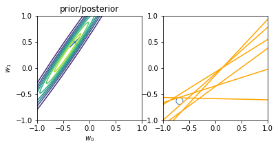
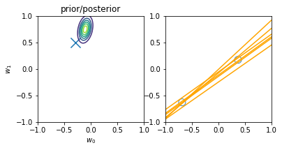
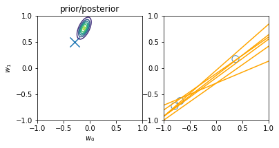
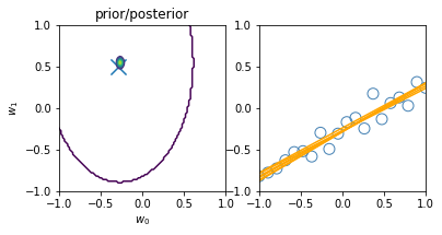
illustration of four steps of online learning for the linear model \(y = w_0 + w_1x\). (inspired on fig 3.7, Pattern Classification and Machine Learning, Chris Bishop)
We start with the prior knowledge that both weights (\(w_0\) and \(w_1\)) are zero-centered, i.e. mean 0, and a std deviation of 1. When a new datapoint is introduced (blue circle on the top-right plot), the new posterior (top-left) is computed from the likelihood and our initial prior. Drawing models from the current priors leads to an innacurate regression model (yellow lines on the top-right plot) Another point is then introduced (2nd row, right), leading to a new posterior (second row, left), computed from the likelihood and the prior (i.e. the posterior of the previous iteration). The model is now more accurate and the earch space (covariance of the weights) is more reduced (second row, left). After two more iterations, the model is already very accurate with a reduce variance on the weights (bottom left) and better-tunned linear regression models (bottom right).
Predictive Variance
Remember that we wanted to model a noisy output defined by \(y = Xw + \varepsilon\) with model parameters \(w \thicksim \mathcal{N}(\mu, \sigma^2)\) and noise parameter \(\varepsilon \thicksim \mathcal{N}(0, \sigma^2)\). The closed-form solution that computes the distribution of \(w\) was provided on the previous section. We’ll now compute the distribution of \(\varepsilon\). Note that drawing samples from the posterior \(p(y \mid X, w, \sigma^2)\) is equivalent to drawing samples from \(y = Xw + \varepsilon\).
We can then compute the expectation of \(y\) as:
\[\begin{align*} \mathbf{E} \left[ y \right] & = \mathbf{E} \left[ X^Tw + \varepsilon \right] \\ & = X^T \mathbf{E} \left[ w \right] + \mathbf{E} \left[ \varepsilon \right] \\ & = X^T m_N \\ \end{align*}\]i.e. because noise has a mean zero, it’s a result equivalent to a linear regression where the weights are set to the close-form solution of their mean value. The variance of \(y\) follows analogously (see Variance rules at the end of the post if in doubt):
\[\begin{align*} \mathbf{Var} \left[ y \right] & = \mathbf{Var} \left[ Xw + \varepsilon \right] \\ & = \mathbf{Var} \left[ Xw \right] + \mathbf{Var} \left[ \varepsilon \right] + 2\mathbf{Cov} \left[ X^Tw, \varepsilon \right] \\ & = \mathbf{Var} \left[ Xw \right] + \mathbf{Var} \left[ \varepsilon \right] & \text{(independent variables)}\\ & = X^T \mathbf{Var} \left[ w \right] X + \mathbf{Var} \left[ \varepsilon \right] & \text{(Var linear transformation, rule 6))}\\ & = X^T S_N X + \sigma^2 & ( \varepsilon \thicksim \mathcal{N}(0, \sigma^2 ) \text{ and noise variance } \sigma^2 \text{)}\\ \end{align*}\]Similarly to the visualization displayed before, introducing new datapoints improves the accuracy of our model:
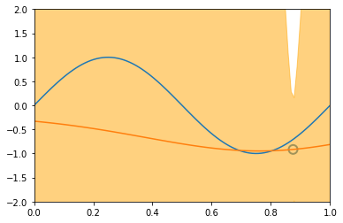
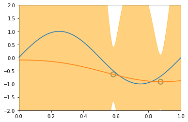
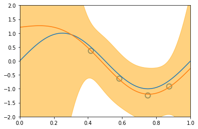
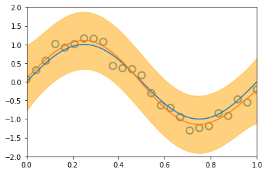
illustration of four steps modelling a synthetic sinusoidal data. Pictures with blue groudntruth, red model mean approximation, and light-orange area of predictive variance. (inspired on fig 3.8, Pattern Classification and Machine Learning, Chris Bishop)
Comparing two Bayesian models
If we want to compare two probabilistic models \(M_1,M_2\), with posteriors given the same dataset \(D\), we compute the ratio of the posteriors, a.k.a. the posterior odds as:
\[\frac{M_1}{M_2} = \frac{ \frac{p(D \mid M_1) \, p(M_1)}{p(D)} }{ \frac{p(D \mid M_2) \, p(M_2)}{p(D)} } = \frac{p(D \mid M_1) \, p(M_1)}{p(D \mid M_2) \, p(M_2)}\]If we assume the same prior for both models, then the equation simplifies to \(\frac{p(D \mid M_1)}{p(D \mid M_2)}\). If this ratio is greater than \(1\), we pick model \(M_1\), otherwise we pick model \(M_2\).
Final Remarks
For more advanced topics on Bayesian Linear Regression refer to chapter 3 in Pattern Recognition and Machine Learning book from Chris Bishop and chapter 9.3 in Mathematics for Machine Learning, both available on the resources page. To download the source code of the closed-form solutions and reproduce the examples above, download the Bayesian Linear Regression notebook.
Finally, it has been shown that a kernelized Bayesian Linear Regression with the Kernel \(K(x, x′)=x^Tx′\) is equivalent to a Gaussian Process.
Misc: linear models of the exponential family
For a set up related to an output which is non-Gaussian but is a member of the exponential family, check Generalized Linear Models.
Appendix: refresher on Linear Algebra
Here are the list of algebraic rules used in this document. For further details, check The Matrix Cookbook for a more detailed list of matrix operations.
- Multiplication:
- \(A(BC) = (AB)C\);
- \(A(B+C)=AB+AC\);
- \((B+C)A=BA+CA\);
- \(r(AB)=(rA)B=A(rB)\) for a scalar \(r\);
- \(I_mA=AI=AI_n\);
- \((A+B)^2 = (A+B)(A+B)^T\);
- \((y - Xw)^2 = (y-Xw)^T(y-Xw)\).
- Transpose:
- \((A^T)^T = A\);
- \((A+B)^T=A^T+B^T\);
- \((rA)^T = rA^T\) for a scalar \(r\);
- \((AB)^T=B^TA^T\);
- Division:
- if \(rA=B\), then \(r=BA^{-1}\), for a scalar \(r\);
- if \(Ar=B\), then \(r=A^{-1}B\), for a scalar \(r\);
- \(Ax=b\) is the system of linear equations \(a_{1,1}x_1 + a_{1,2}x_2 + ... + a_{1,n}x_n = b_1\) for row \(1\), repeated for every row;
- therefore, \(x = A^{-1}b\), if matrix has \(A\) an inverse;
- Inverse:
- \(AA^{-1}=A^{-1}A=I\);
- If \(A\) is invertible, its inverse is unique;
- If \(A\) is invertible, then \(Ax=b\) has an unique solution;
- If \(A\) is invertible, \((A^{-1})^{-1}=A\);
- \(rA^{-1} = (\frac{1}{r}A)^{-1}\) for a scalar \(r\);
- First Order derivatives:
- \(\frac{d w^TX}{dw} = \frac{d X^Tw}{dw} = X\);
- \(\frac{d X^TwY}{dw} = XY^T\);
- \(\frac{d X^Tw^TY}{dw} = YX^T\);
- \(\frac{d X^TwX}{dw} = \frac{d X^Tw^TX}{dw} = XX^T\);
- Variance and Covariance:
- \(\mathbb{Var}(X) = \mathbb{Cov}(X,X)\);
- \(\mathbb{Var}(rX) = r \mathbb{Var}(X)\), for scalar \(r\);
- \(\mathbb{Var}(X+Y) = \mathbb{Var}(X) + \mathbb{Var}(Y) + 2\mathbb{Cov}(X,Y)\);
- \(\mathbb{Var}(X+Y) = \mathbb{Var}(X) + \mathbb{Var}(Y)\), if X and Y are independent (ie, zero covariance);
- \(\mathbb{Var}(X) = \mathbf{E}[(X-\mathbf{E}[X])^2 ] = \mathbf{E} \left[ X^2 - 2X\mathbf{E}[X] + \mathbf{E}[X]^2 \right] = \mathbf{E}[X^2] - 2\mathbf{E}[X]\mathbf{E}[X] + \mathbf{E}[X]^2 = \mathbf{E}[X^2] - \mathbf{E}[X]^2\);
- If \(y\) is a linear transformation of univariate form \(y=mx+b\) or multivariate form \(y=Xw+b\) then:
- Variance in univariate form: \(\mathbb{Var}(y)=m^2 \,\, \mathbb{Var}(w)\);
- Variance in multivariate form: \(Var (Xw + b) = Var (Xw) = X \mathbb{Var}(w) X^T = X \Sigma X^T\), where \(\Sigma\) is the covariance matrix of \(X\);
- Expected Value in multivariate form: \(\mathbf{E}[Xw + b] = X \mathbf{E}[w] + b = X \mu + b\), where \(\mu\) is the mean of \(X\)
- formulas 6.50 and 6.51 in Mathematics for Machine Learning