Closed-form Linear Regression and Matrix Factorization, and loss functions
Regression relates an input variable to an output, to either predict new outputs, or understand the effect of the input in the output. A regression dataset consists of a set of pairs \((x_n, y_n)\) of size \(N\) with input \(x_n\) and output/label \(y_n\). For a new input \(x_n\), the goal of regression is to find \(f\) such that \(y_n \approx f(x_n)\). If we wan’t to fit the dataset to a multidimensional plane, we are solving the (multivariate) linear regression problem, by finding the weights \(w\) that approximate \(y_n\) i.e:
\[y_n \approx f(x_n) = w_0 + w_1 x_{n1} + ... + + w_D x_{nD} \hspace{1cm}\text{, or simply}\hspace{1cm} y_n \approx f(X) = Xw.\]We use an error or loss function \(L(w)\) to indicate how good our estimation is. As as example, the Mean Squared Error (MSE) loss is described as \(L(w) = \frac{1}{N} \sum_{n=1}^N [ y_n - f(x_n)]^2\), and has the property of penalizing predictions with larger errors due to the square term. Another loss function, the Mean Absolute Error (MAE), with \(L(w) = \frac{1}{N} \sum_{n=1}^N \mid y_n - f(x_n) \mid\), enforces sparsity in the weight values.
In brief, we want to find the weight values that mimimize the loss function. A naive approach is the Grid Search, a brute-force approach that tests all combinations of \(w\) in a given interval. This is usually a dull approach and only works on very low dimensionality problems. An alternative is to optimize the loss function by computing the gradient of the derivative and stepping \(w\) to the values that minimizes the loss. The most common methods are the gradient descent and its variants:
- Gradient Descent: \(w^{t+1} = w^{t} - \gamma \triangledown L (w^t)\), for step size \(\gamma\), and gradient \(\triangledown L (w) = [ \frac{\partial L(w)}{\partial w_1}, ... , \frac{\partial L(w)}{\partial w_D} ]^T\);
- Stochastic Gradient Descent: \(w^{t+1} = w^{t} - \gamma \triangledown L_n (w^t)\), for a random choice of an inputs \(n\). Computationally cheap but unbiased estimate of gradient;
- Mini-batch SGD: \(w^{t+1} = w^{t} - \gamma \frac{1}{\mid B \mid} \sum_{n \in B} \triangledown L_n (w^t)\), for a random subset \(B \subseteq [N]\). For each sample \(n\) , we compute the gradient at the same current point \(w^{(t)}\);
For the particular example of linear regression and the Mean Squared Error loss function, the problem is called Least Squares and has a closed-form solution. In practice, we want to minimize the following:
\[\begin{align*} (y - Xw)^2 = \, & (y-Xw)^T(y-Xw) \\ = \, & y^Ty - y^TXw - (Xw)^Ty + (Xw)^TXw \\ = \, & y^Ty - w^TX^Ty - w^TX^Ty + w^TX^TXw \\ = \, & y^Ty - 2 w^TX^Ty + w^TX^TXw\\ \end{align*}\]We want to compute the \(w\) that minimizes the loss, or equivalently, where its derivative is 0. So we compute:
\[\begin{align*} & \frac{\partial}{\partial w} y^Ty - 2 w^TX^Ty + w^TX^TXw = 0 \\ \Leftrightarrow \, & 0 - 2 X^Ty + 2 X^TXw = 0 \\ \Leftrightarrow \, & 2 X^TXw = 2X^Ty \\ \Leftrightarrow \, & w = (X^TX)^{-1} X^Ty\\ \end{align*}\]Note that we used the trick \(\frac{\partial w^Ta}{\partial w} = \frac{\partial a^Tw}{\partial w} = a\) (The Matrix Cookbook, eq 2.4.1). The results tells us that if \(X^TX\) is invertible, this minimization problem has an unique closed-form solution given by that final form. As a side note, the Gram matrix \(X^TX\) is invertible if X has full column rank, i.e. \(rank(X)=D\) (we’ll ommit the proof). The rank of a matrix is defined as the maximum number of linearly independent column vectors in the matrix, therefore we assume that all columns are linearly independent.
Regularization
It’s a common practice to add to the loss a regulatization term \(\Omega\) that penalizes complex models. Therefore our loss minimization problem becomes:
\[min_w L(w) + \Omega (w)\]Common regularizer approaches are:
- L1 regularization: \(\Omega(w) = \lambda \mid w \mid\), where \(\mid w \mid = \sum_{i=0}^M \mid w_i \mid\)
- this is called LASSO Regression as in Least Absolute Shrinkage and Selection Operator.
- the parameter \(\lambda \gt 0\) can be tuned to reduce overfitting. This is the model selection problem.
- encourages simple, sparse models (i.e. models with fewer parameters). This particular type of regression is well-suited for models showing high levels of muticollinearity or when you want to automate certain parts of model selection, like variable selection/parameter elimination.
- L2 regularization (standard Euclidean norm): \(\Omega(w) = \lambda \| w \|^2\), where \(\| w \|^2 = \sum_{i=0}^M w_i^2\)
- Large weights will be penalized, as they are considered unlikely;
- If \(L\) is the MSE, this is called Ridge Regression ;
- similarly to the Least Squares problem, the loss of the MSE with Rigde Regression has an analytical solution:
- computed by minimizing \((y - Xw)^T(y-Wx) + \lambda w^Tw\), and;
- derivating with respect to \(w\) leads to the normal equation \(w = (X^TX - \lambda I)^{-1} X^Ty\).
Note: in statistics, shrinkage is the reduction in the effects of sampling variation, e.g. data overfitting to train data and not performing well on unseen data. Regularization attempts to do this by “shrinking” model parameters towards 0 in LASSO or to make model parameters smaller in Ridge Regression.
Other techniques that do not add the regularizer term to the loss function but helps in improving model accuracy:
- dropout: a method to drop out (ignore) neurons in a (deep) neural network at every batch during training and using all neurons at validation. Shown to increase generalization by forcing the model to train wihtout relying on specific weights. (see separate post for more details.
- layer, instance, batch, and group normalization: methods to reduce internal covariance shift by fitting the output of activation layers to a standard normal distributed. Learns optional scale and shift parameters that scale of standard deviation and shift of mean for improved performance over the standard normal distribution.
Matrix Factorization
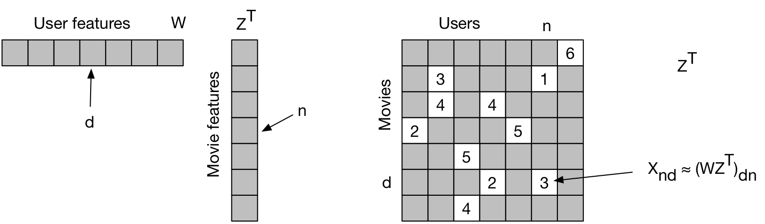
Matrix factorization can be used to discover underling latent factors and/or to predict missing values of the matrix. We aim to find \(W\), \(Z\) such that \(W \approx WZ^T\). I.e. we aim to predict \(x_{dn}\), where \(d\) is an element in \(Z\), and \(n\) is an element in \(W\). For movie rating, \(Z\) could be users, \(W\) could be movies, and \(x_{dn}\) the star rating.
We aim at optimizing:
\[min_{W,Z} L (W,Z) = \frac{1}{2} \sum_{(d,n) \in \Omega} [ x_{dn} - (WZ^T)_{dn}]^2\]where \(D \in R^{D \times K}\) and \(Z \in R^{N \times K}\) are tall matrices, and \(\Omega \subseteq [D] \times [N]\) collects the indices of the observed ratings of the input matrix \(X\).
This cost function is not convex and not identifiable. \(K\) is the number of latent features (e.g. gender, age group, citizenship, etc). Large \(K\) facilitates overfitting. We can add a regularizer to the function:
\[min_{W,Z} L (W,Z) = \frac{1}{2} \sum_{(d,n) \in \Omega} [ x_{dn} - (WZ^T)_{dn}]^2 + \frac{\lambda_w}{2} \| W \|^2 + \frac{\lambda_z}{2} \| Z \|^2\]where (again), \(\lambda_z\) and \(\lambda_w\) are scalars.
We use stochastic gradient descent to optimize this problem. The training objective is a function over |\(\Omega\)| terms (one per rating):
\[\frac{1}{| \Omega |} \sum_{(d,n) \in \Omega} \frac{1}{2} [x_{dn} - (WZ^T)_{dn}]^2\]For one fixed element \((d,n)\), we derive the gradient \((d',k)\) for \(W\) and \((n',k)\) for \(Z\):
\[(d',k) = \frac{\partial}{\partial w_{d',k}} \frac{1}{2} [x_{dn} - (WZ^T)_{dn}]^2 = \begin{cases} -[x_n - (WZ^T)_{dn}] z_{n,k} & \text{, if } d'=d\\ 0, & \text{, otherwise} \end{cases}\]and
\[(n',k) = \frac{\partial}{\partial w_{n',k}} \frac{1}{2} [x_{dn} - (WZ^T)_{dn}]^2 = \begin{cases} -[x_n - (WZ^T)_{dn}] w_{d,k} & \text{, if } n'=n\\ 0, & \text{, otherwise} \end{cases}\]Reminder: \(z_{n,k}\) are user features, \(w_{d,k}\) are movie features. The gradient has \((D+N)K\) entries.
We can also use Alternating Least Squares (ALS). The ALS factorizes a given matrix \(R\) into two factors \(U\) and \(V\) such that \(R \approx U^TV\).
-
If there are no missing ratings in the matrix ie \(\Omega = [D] \times [N]\), then:
\[\begin{align*} min_{W,Z} L(W,Z) = & \frac{1}{2} \sum_{d=1}^D \sum_{n=1}^N [x_{dn} - (WZ^T)_{dn}]^2 + \text{ (regularizer) } \\ = & \frac{1}{2} \| X - WZ^T \| ^2 + \frac{\lambda_w}{2} \| W \|^2 + \frac{\lambda_z}{2} \| Z \|^2 \end{align*}\]- We can use coordinate descent (minimize \(W\) for fixed \(Z\) and vice-versa) to minimize cost plus regularizer;
-
If there are missing entries, the problem is harder, as only the ratings \((d,n) \in \Omega\) contribute to the cost, i.e..;
\[min_{W,Z} L(W,Z) = \frac{1}{2} \sum_{(d,n) \in \Omega} [x_{dn} - (WZ^T)_{dn}]^2 + ...\]
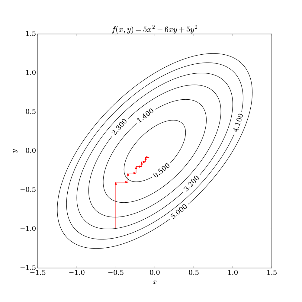
Coordinate Descent
The coordinate descent optimization method iterates over individual coordinates (keeping others fixed), in order to minimize the loss function.
source: wikipedia
The main advantage is that it is extremely simple to implement and doesn’t require any knowledge of the derivative of the function. It’s really useful for extremely complicated functions or functions whose derivatives are far more expensive to compute than the function itself. However, due to its iterative nature, it’s not a good candidate for parallelism. Another issue is that it has a a non-smooth multivariable function, thus it may be stuck in non-stationary point if the level curves of a function are not smooth (source: wikipedia).
Risk and Loss Functions
In ML, on non-probabilistic models, we follow the principle of empirical risk empirical risk minimization, in order to find good parameters. The risk is the expected loss between the expected output \(y_n\) and the predicted value \(\hat{y}_n\), ie
\[r(f) = \mathbb{E}[l(\hat{y}_n, y_n)]\]where the predictor \(\hat{y}_n = f(x_n, \theta∗)\) represents the output of the model \(f\) with input data \(x_n\) and parameters \(\theta*\).
On the case of a statistical model, the object of the maximum likelihood estimator is to find the function of the parameters that fits the model well
\[L_x(θ) = −log p(x | θ) .\]We’ll omit details on likelihood estimators, as they are covered in a different post.
Mean Squared Error
Most regression tasks use the Mean Squared Error loss function:
\[MSE(\hat{y}_n) = \mathbb{E}\left[ (y_n - \hat{y}_n)^2 \right].\]or the Mean Absolute Error, similar to MSE but uses the absolute value instead of the squared value of the difference in \(y\) and \(\hat{y}\).
Cross-Entropy
The cross-entropy is equivalent to the negative of the log-likelihood (of the softmax when output of the model is not a distribution). However, for classification tasks, we use the cross-entropy formulation avoid numerical instabilities and overflows. Most classification tasks use the binary or multi-class cross-entropy loss functions:
- binary: \(H(p) = -(y \log p(x) + (1-y) \log (1-p(x)))\), i.e. it simplifies to \(-\log p(x)\) for true label \(y=1\), and to \(-\log (1-p(x))\) for true label \(y=0\).
- multi-class: \(H(p,q) = -\sum_x p(x) \log(q(x))\), for true value \(p\) and predicted value \(q\).
Triplet Loss
Triplet loss is used on classification tasks where the number of classes is very large. Triplet loss helps by learning distributed embeddings representation of data points in a way that in the high dimensional vector space, contextually similar data points are projected in the near-by region whereas dissimilar data points are projected far away from each other. The network is trained against triplets of images: an anchor image of a person, positive image which is another image of the same person, and a negative image which is a picture of another person. The Triplet Loss minimizes the euclidian distance between an anchor and a positive and maximizes the distance between the Anchor and the negative. Tasks that we can perform: face recognition (“who’s this person”) and validation (“are these the same person?”) and clustering (“find most similar people”). The formulation is:
\[{\displaystyle {\mathcal {L}}\left(A,P,N\right)=\operatorname {max} \left({\|\operatorname {f} \left(A\right)-\operatorname {f} \left(P\right)\|}^{2}-{\|\operatorname {f} \left(A\right)-\operatorname {f} \left(N\right)\|}^{2}+\alpha ,0\right)}\]where \(A\) is an anchor input, \(P\) is a positive input of the same class as \(A\), \(N\) is a negative input of a different class from \(A\), \(\alpha\) is a margin between positive and negative pairs, and \(f\) is an embedding. For more details see the original paper FaceNet: A Unified Embedding for Face Recognition and Clustering.
Contrastive Loss
Contrastive loss is similar and often confused with triplet loss. Yet these solve different problems: for known similarity relationships, we use Contrastive loss. For only negative/positive relationships (like for face recognition where people’s identity is the anchor), then Triplet loss is used. In practice, the triplet loss considers the anchor-neighbor-distant triplets while the contrastive loss deals with the anchor-neighbor and anchor-distant pairs of samples. The contrastive loss trains siamese networks against pairs of inputs labelled as similar or dissimilar (1 or 0). Contrastive loss is formulated in terms of the similarity label \(y\) (1 for similar, 0 for assimilat), and the euclidian distance between two images \(D\) as:
\[L = \frac{1}{2} ⋅y⋅D + \frac{1}{2} ⋅(1−y)⋅max(0,m−D)^2\]where \(m\) is a hyper-parameter. For the original paper refer to Dimensionality Reduction by Learning an Invariant Mapping or my summary in the publications bookmark.
Connectionist Temporal Classification loss
Connectionist Temporal Classification (CTC) is a classifier and loss function for noisy sequential unsegments input data, for training recurrent neural networks (RNNs) such as LSTM networks to tackle sequence problems where the timing is variable. Published on Connectionist Temporal Classification: Labelling Unsegmented Sequence Data with Recurrent Neural Networks. Already summarized in the publications bookmark section.
Focal Loss
Focal Loss is an extension of Cross-Entropy Loss designed to address class imbalance, a common issue in e.g. medical image segmentation where the background (non-lesion regions) is much more prevalent than the foreground (lesion regions). Focal Loss focuses on hard-to-classify examples and down-weights the loss contribution from easy examples.
\[\mathcal{L}_{\text{focal}} = -\alpha (1 - p_t)^\gamma \log(p_t)\]where:
- \(p_t\) is the model’s estimated probability for the true class.
- \(α\) is a balancing factor to adjust the weight of the positive class (especially useful for imbalanced datasets).
- \(γ\) is the focusing parameter, usually set to 2, which adjusts the focus on hard-to-classify examples.
For multi-class classification, Focal Loss can be generalized as:
\[\mathcal{L}_{\text{focal}} = -\alpha_t (1 - p_t)^\gamma \log(p_t)\]where \(\alpha_t\) is the balancing factor for class \(t\).
Dice Loss
Dice loss (or Dice Similarity Coefficient Loss) is a loss function used specifically for image segmentation tasks, especially when evaluating the overlap between predicted and ground truth segmentation masks. It measures the similarity between two sets, with values ranging from 0 (no overlap) to 1 (perfect overlap). Dice Loss is typically used when precise object boundaries are important, such as segmenting organs, tumors, or any region of interest in medical imaging where the goal is to accurately delineate the object of interest from the surrounding tissue. Key benefits of Dice Loss:
- Direct Focus on Overlap: Dice loss directly optimizes the overlap between predicted and ground truth masks, which is crucial for segmentation tasks where precise boundary delineation matters.
- Effective for Imbalanced Classes: It works well when there is a significant class imbalance between foreground and background, as it evaluates segmentation performance based on the overlap of the foreground regions rather than pixel accuracy.
- Works Well with Small Objects: Dice loss is particularly effective in medical imaging tasks where the objects of interest (e.g., tumors, organs) might occupy a small portion of the image.
Where:
- \(A\) is the set of predicted pixels.
- \(B\) is the set of ground truth pixels.
- \(\mid 𝐴 ∩ 𝐵 \mid\) is the intersection of the predicted and ground truth sets, representing the overlap.
For practical implementation, Dice Loss is often computed as:
\[\mathcal{L}_{\text{Dice}} = 1 - \frac{2 \sum_{i=1}^{N} p_i g_i}{\sum_{i=1}^{N} p_i + \sum_{i=1}^{N} g_i}\]where
- \(𝑝_𝑖\) is the predicted value for the i-th pixel.
- \(𝑔_𝑖\) is the ground truth value for the i-th pixel.
For multi-class segmentation, a generalized form of Dice Loss is:
\[\mathcal{L}_{\text{Dice}} = 1 - \frac{2 \sum_{i=1}^{N} p_i g_i}{\sum_{i=1}^{N} p_i + \sum_{i=1}^{N} g_i}\]where \(N\) is the number of classes.