Exponential Family of Distributions

On the previous post, we saw that computing the Maximum Likelihood estimator and the Maximum-a-Posterior on a normally-distributed set of parameters becomes much easier once we apply the log-trick. The rationale is that since $\log$ is an increasingly monotonic function, the maximum and minimum values of the function to be optimized are the same as the original function inside the $\log$ operator. Thus, by applying the $\log$ function to the solution, the normal distribution becomes simpler and faster to compute, as we convert a product with an exponential into a sum.

However, this is not a property of the Gaussian distribution only. In fact, most common distributions including the exponential, log-normal, gamma, chi-squared, beta, Dirichlet, Bernoulli, categorical, Poisson, geometric, inverse Gaussian, von Mises and von Mises-Fisher distributions can be represented in a similar syntax, making it simple to compute as well. To the set of such distributions we call it the Exponential Family of Distributions, and we will discuss them next.

Detour: relationship between common probability distributions

Probability distributions describe the probabilities of each outcome, with the common property that the probability of all events adds up to 1. They can also be classified in two subsets: the ones described by a probability mass function if specified for discrete values, or probability density functions if described within some continuous interval. There are dozens (hundreds?) of different distributions, even though only 15 of them are often mentioned and used, and have some kind of relationship among themselves:

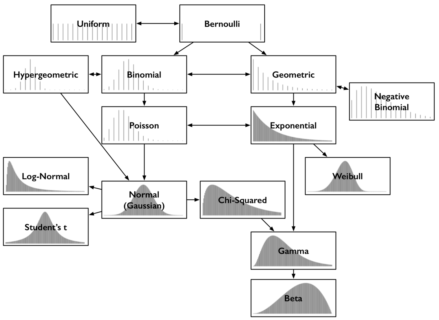
15 most common probability distributions and their relationships. (source: post Common probability distributions from Sean Owen)

A bried summary of their relationship follows. For more details, check the original post from Sean Owen:

Bernoulli and Uniform: the uniform distribution yields equal probability to each discrete outcome e.g. a coin toss or a dice roll; the Bernoulli yields an unequal probability to two discrete outcomes as $p$ and $1-p$, e.g. an unfair coin toss;
Binomial and Hypergeometric: the binomial can be seen as the probability of the sum of outcomes of what follows a bernoulli distribution, e.g. rolling a dice 30 times, what’s the probability that we get the outcome six? This count follows the binomial distribution, with parameter $n$ trials, and $p$ as success (a la Bernoulli);
Poisson and Binomial: like the binomial distribution, the poisson distribution is a distribution of a count — the number of times some event happened over a discrete time, given a rate for the event to ocur. It’s parametrized as $\lambda = np$ (the $n$ and $p$ parameters of the binomial);
Geometric and Negative Binomial: while in the binomial we count the number of times the probability succeeds in yielding a given event after a number of trial, in the geometric distribution we count how many negative trials until we succeed in out event happening; The negative binomial distribution is a simple generalization of the geometric, measuring the number of failures until $r$ successes have occurred, not just 1;
Exponential and Weibull: the exponential distribution is the geometric on a continuous interval, parametrized by $\lambda$, like Poisson. While it will describes “time until event or failure” at a constant rate, the Weibull distribution models increases or decreases of rate of failures over time (i.e. models time-to-failure);
Normal, Log-Normal, Student’s t, and Chi-squared: if we take a set of values following the same (any) distribution and sum them, that sum of values follows approximatly the normal distribution — this is true regardless of the underlying distribution, and this phenomenon is called the Central Limit Theorem. The log-normal distribution relates to distributions whose logarithm is normally distributed. The exponentiation of a normally distribution is log-normally distributed. Student’s t-distributions are normal distribution with a fatter tail, although is approaches normal distribution as the parameter increases. The chi-square distribution if the distribution of sum-of-squares of normally-distributed values;
Gamma and Beta: the gamma distribution is a generalization of the exponential and the chi-squared distributions. Like the exponential distribution, it is used to model waiting times e.g. the time until next $n$ events occur. It appears in machine learning as the conjugate prior to some distributions. The beta distribution is the conjugate prior to most of the other distributions mentioned here;

Exponential Family of distributions

The exponential family of distribution is the set of distributions parametrized by $\theta \in \mathbf{R}^D$ that can be described in the form:

\[p(x \mid \theta) = h(x) \exp \left(\eta(\theta)^T T(x) -A(\theta)\right) \label{eq_main_theta}\]

or in a more extensive notation:

\[p(x \mid \theta) = h(x) \exp\left(\sum_{i=1}^s \eta_i({\boldsymbol \theta}) T_i(x) - A({\boldsymbol \theta}) \right)\]

where $T(x)$, $h(x)$, $\eta(\theta)$, and $A(\theta)$ are known functions. An alternative notation to equation \ref{eq_main_theta} describes $A$ as a function of $\eta$, regardless of the transformation from $\theta$ to $\eta$. This new expression we call an exponential family in its natural form, and looks like:

\[p(x \mid \eta) = h(x) \exp \left(\eta^T T(x) -A(\eta)\right) \label{eq_main_eta}\]

The therm $T(x)$ is a sufficient statistic of the distribution. The sufficient statistic is a function of the data that holds all information the data $x$ provides with regard to the unknown parameter values;

The intuitive notion of sufficiency is that $T(X)$ is sufficient for $\theta$, if there is no information in $X$ regarding $\theta$ beyond that in $T(X)$. That is, having observed $T(X)$, we can throw away $X$ for the purposes of inference with respect to $\eta$;
Moreover, this means that the likelihood ratio is the same for any two datasets $x$ and $y$, i.e. if $T(x)=T(y)$, then $\frac{p(x \mid \theta_1)}{p(x \mid \theta_2)} = \frac{p(y \mid \theta_1)}{p(y \mid \theta_2)}$;

The term $\eta$ is the natural parameter, and the set of values $\eta$ for which $p(x \mid \theta)$ is finite is called the natural parameter space and is always convex;

The term $A(\eta)$ is the log-partition function because it is the logarithm of a normalization factor, ensuring that the distribution $f(x;\mid \theta)$ sums up or integrates to one (without wich $p(x \mid \theta)$ is not a probability distribution), ie.:

\[A(\eta) = \log \int_x h(x) \exp (\eta^T T(x)) \, \mathrm{d}x;\]

Another important point is that the mean and variance of $T(x)$ can be derived by differentiating $A(\eta)$ and computing the first- and second- derivative, respectively:

\[\begin{align*} \frac{dA}{d\eta^T} & = \frac{d}{d\eta^T} \left( \log \int_x h(x) \exp (\eta^T T(x)) \, \mathrm{d}x \right) \\ & = \frac{ \int_x T(x) h(x) \exp (\eta^T T(x)) \, \mathrm{d}x}{\int_x h(x) \exp (\eta^T T(x)) \, \mathrm{d}x} &\text{log derivative rule:} \left(\frac{d}{dx} log(x) = \frac{x'}{x}\right) \\ & = \int_x T(x) h(x) exp(\eta^TT(x) - A(\eta)) \, \mathrm{d}x & \text{(definition of } p(x \mid \eta) \text{, and } \frac{∫f \, dx}{∫g \, dx} = ∫(f - g ) \, dx \text{)}\\ & = \mathbf{E}[T(X)] & (\text{def. expected value: } \mathbf{E}[X] = \int_x x \, f(x) dx \text{, for density func. } f(x))\\ \end{align*}\]

For the complete dataset $X=(x_1, x_2, ..., x_m$)$. I.e. the first derivative of$A(\eta)$$ is equal to the mean of the sufficient statistic. We can now look at the second derivative:

\[\begin{align*} \frac{d^2A}{d\eta\,d\eta^T} & = \int_x h(x) T(x) \left( T(x) -\frac{d}{d\eta^T}A(\eta)\right)^T \, exp\left(\eta^TT(x) - A(\eta)\right) \, dx \\ & = \int_x h(x) T(x) \left( T(x) - \mathbf{E}[T(X)] \right)^T \, exp\left(\eta^TT(x) - A(\eta)\right) \, dx & (\frac{dA}{d\eta^T} = \mathbf{E}[T(X)])\\ & = \mathbf{E}[T(X)T(X)^T] -\mathbf{E}[T(X)] \, \mathbf{E}[T(X)]^T & (\mathbf{E}[X] = \int_x x \, f(x) dx)\\ & = \mathbf{Var}[T(X)] & (Var(X)=E[X^2]-E[X]^2)\\ \end{align*}\]

and as expected the second derivative is equal to the variance of $T[X]$.

One requirement of the exponential family distributions is that the parameters must factorize (i.e. must be separable into products, each of which involves only one type of variable), as either the power or base of an enxponentiation operation. I.e. the factors must be one of the following:

\[f(x), g(\theta), c^{f(x)}, c^{g(\theta)}, {[f(x)]}^c, {[g(\theta)]}^c, {[f(x)]}^{g(\theta)}, {[g(\theta)]}^{f(x)}, {[f(x)]}^{h(x)g(\theta)}, \text{ or } {[g(\theta)]}^{h(x)j(\theta)}\]

where $f$ and $h$ are arbitrary functions of $x$, $g$ and $j$ are arbitrary functions of $\theta$; and c is an arbitrary constant expression.

Another important point is that a product of two exponential-family distributions is as well part of the exponential family, but unnormalized:

\[\left[ h(x) \exp \left(\eta^T T(x) -A(\eta_1)\right) \right] * \left[ h(x) \exp \left(\eta^T T(x) -A(\eta_1)\right) \right] = \widetilde{h}(x) \exp \left(\left(\eta_1+\eta_2\right)^T T(x) -\widetilde{A}(\eta_1, \eta_2)\right)\]

Finally, the exponential family distribution have conjugate priors (i.e. prior and posterior distributions have distributions from the exponential family), and the posterior predictive distribution has always a closed-form solution (provided that the normalizing factor can also be stated in closed-form), both important properties for Bayesian statistics.

Example: Univariate Gaussian distribution

The univariate Gaussian distribution is defined for an input $x$ as:

\[p(x \mid \mu, \sigma^2 ) = \frac{1}{ \sqrt{2 \pi \sigma^2} } \,\, exp \left( - \frac{(x - \mu)^2}{2 \sigma^2} \right)\]

for a distribution with mean $\mu$ and standard deviation $\sigma$. By moving the terms around we get:

\[\begin{align*} %% source: http://www.cs.columbia.edu/~jebara/4771/tutorials/lecture12.pdf p(x \mid \mu, \sigma ) & = \frac{1}{ \sqrt{2 \pi \sigma^2} } \,\, exp \left( - \frac{(x - \mu)^2}{2 \sigma^2} \right) \\ & = \frac{1}{ \sqrt{2 \pi } } \,\, exp \left( - \log \theta - \frac{x^2}{2 \sigma^2} + \frac{\mu x}{\sigma^2} - \frac{\mu^2}{2 \sigma^2} \right) \\ & = \frac{1}{ \sqrt{2 \pi } } \,\, exp \left( \theta^TT(x) - \log \theta - \frac{\mu}{2\sigma^2} \right) \\ & = h(x) \,\, exp \left( \eta(\theta)^TT(x) - A(\theta) \right) \\ \end{align*}\]

where:

$h(x) = \frac{1}{ \sqrt{2 \pi}}$,
$T = { x \choose x^2 }$,
$\eta(\theta) = { \mu/(\sigma^2) \choose -1/(2\sigma^2) }$,
$A(\eta) = \frac{\mu^2}{2\sigma^2} + \log \sigma = - \frac{ \eta^2_1}{4 \eta_2} - \frac{1}{2} \log(-2\eta_2)$,

We will now use the first and second derivative of $A(x)$ to compute the mean and the variance of the sufficient statistic $T(x)$:

\[\begin{align*} %% source: https://people.eecs.berkeley.edu/~jordan/courses/260-spring10/other-readings/chapter8.pdf \frac{dA}{d\eta_1} & = \frac{dA}{d\eta_1} \left( - \frac{ \eta^2_1}{4 \eta_2} - \frac{1}{2} \log(-2\eta_2) \right) \\ & = \frac{\eta_1}{2\eta_2} \\ & = \frac{\mu / \sigma^2}{1/\sigma^2} \\ & = \mu \\ \end{align*}\]

which is the mean of $x$, the first component of the sufficient analysis. Takes the second derivative we get:

\[%% source: https://people.eecs.berkeley.edu/~jordan/courses/260-spring10/other-readings/chapter8.pdf \frac{d^2A}{d\eta_1^2} = - \frac{1}{2\eta_2} = \sigma^2\]

which is the standard deviation of our normal distribution, by definition.

Example: Bernoulli distribution

Similarly, to compute the exponential family parameters in the Bernoulli distribution we follow as:

\[%% source: http://www.cs.columbia.edu/~jebara/4771/tutorials/lecture12.pdf \begin{align*} p(x, \alpha) & = \alpha^x (1-\alpha)^{1-x} \hspace{0.5cm}, x \in \{0,1\} \\ & = \exp \left( \log (\alpha^x (1-\alpha)^{1-x} \right) \\ & = \exp \left( x \log \alpha + (1-x) \log (1-\alpha) \right) \\ & = \exp \left( x \log \frac{\alpha}{1-\alpha} + \log (1-\alpha) \right) \\ & = \exp \left( x \eta - \log (1+e^\eta) \right) \\ \end{align*}\]

where:

$h(x) = 1$,
$T(x) = x$,
$\eta = \log \frac{\alpha}{1-\alpha}$,
$A(\eta) = \log ( 1+e^\eta)$.

We now compute the mean of $T(x)$ as:

\[\begin{align*} \frac{d A}{d \eta} = \frac{e^\eta}{1+e^\eta} = \frac{1}{1 + e^{-\eta}} = \mu \\ \end{align*}\]

which is the mean of a Bernoulli variable. Taking a second derivative yields:

\[%% source: https://people.eecs.berkeley.edu/~jordan/courses/260-spring10/other-readings/chapter8.pdf \frac{d^2A}{d\eta^2} = \frac{d \mu}{d \eta} = \mu (1-\mu)\]

which is the variance of a Bernoulli variable.

Parameters for common distributions

The following table provides a summary of most common distributions in the exponential family and their exponential-family parameters. For a more exhaustive list, check the Wikipedia entry for Exponential Family.

Distribution	Probability Density/Mass Function	Natural parameter(s) $\boldsymbol\eta$	Inverse parameter mapping	Base measure $h(x)$	Sufficient statistic $T(x)$	Log-partition $A(\boldsymbol\eta)$	Log-partition $A(\boldsymbol\theta)$
Bernoulli distribution	$f(x ; p) = p^x (1-p)^{1-x}$	$\log\frac{p}{1-p}$ (logit function)	$\frac{1}{1+e^{-\eta}} = \frac{e^\eta}{1+e^{\eta}}$ (logistic function)	$1$	$x$	$\log (1+e^{\eta})$	$-\log (1-p)$
binomial distribution with known number of trials n	$f(x; n,p) = \binom{n}{x}p^x(1-p)^{n-x} $	$\log\frac{p}{1-p}$	$\frac{1}{1+e^{-\eta}} = \frac{e^\eta}{1+e^{\eta}}$	${n \choose x}$	$x$	$n \log (1+e^{\eta})$	$-n \log (1-p)$
Poisson distribution	$ f(x; \lambda)=\frac{\lambda^x e^{-\lambda}}{x!}$	$\log\lambda$	$e^\eta$	$\frac{1}{x!}$	$x$	$e^{\eta}$	$\lambda$
negative binomial distribution with known number of failures r	$ f(x; r, p) = \binom{x+r-1}{x} p^r(1-p)^x $	$\log p$	$e^\eta$	${x+r-1 \choose x}$	$x$	$-r \log (1-e^{\eta})$	$-r \log (1-p)$
exponential distribution	$ f(x;\lambda) = \begin{cases} \lambda e^{-\lambda x} & x \ge 0, \\ 0 & x < 0. \end{cases} $	$-\lambda$	$-\eta$	$1$	$x$	$-\log(-\eta)$	$-\log\lambda$
Pareto distribution with known minimum value $ x_m $	$ \overline{f}(x;\alpha) = \Pr(X>x) = \\ \begin{cases} \left(\frac{x_\mathrm{m}}{x}\right)^\alpha & x\ge x_\mathrm{m}, \\ 1 & x < x_\mathrm{m}, \end{cases} $	$-\alpha-1$	$-1-\eta$	$1$	$\log x$	$-\log (-1-\eta) + (1+\eta) \log x_{\mathrm m}$	$-\log \alpha - \alpha \log x_{\mathrm m}$
Laplace distribution with known mean μ	$ f(x ; \mu,b) = \frac{1}{2b} \exp \left( -\frac{\|x-\mu\|}{b} \right) \\ = \frac{1}{2b} \left\{\begin{matrix} \exp \left( -\frac{\mu-x}{b} \right) & \text{if }x < \mu \\[8pt] \exp \left( -\frac{x-\mu}{b} \right) & \text{if }x \geq \mu \end{matrix}\right. $	$-\frac{1}{b}$	$-\frac{1}{\eta}$	$1$	$\|x-\mu\|$	$\log\left(-\frac{2}{\eta}\right)$	$\log 2b$
normal distribution known variance	$ f(x; \mu, \sigma^2) = \frac{1}{\sigma \sqrt{2\pi} } e^{-\frac{1}{2}\left(\frac{x-\mu}{\sigma}\right)^2} $	$\mu/\sigma$	$\sigma\eta$	$\frac{e^{-\frac{x^2}{2\sigma^2}}}{\sqrt{2\pi}\sigma}$	$\frac{x}{\sigma}$	$\frac{\eta^2}{2}$	$\frac{\mu^2}{2\sigma^2}$
normal distribution	$ f(x; \mu, \sigma^2) = \frac{1}{\sigma \sqrt{2\pi} } e^{-\frac{1}{2}\left(\frac{x-\mu}{\sigma}\right)^2} $	$\begin{bmatrix} \dfrac{\mu}{\sigma^2} \\[10pt] -\dfrac{1}{2\sigma^2} \end{bmatrix}$	$\begin{bmatrix} -\dfrac{\eta_1}{2\eta_2} \\[15pt] -\dfrac{1}{2\eta_2} \end{bmatrix}$	$\frac{1}{\sqrt{2\pi}}$	$\begin{bmatrix} x \\ x^2 \end{bmatrix}$	$-\frac{\eta_1^2}{4\eta_2} - \frac12\log(-2\eta_2)$	$\frac{\mu^2}{2\sigma^2} + \log \sigma$
lognormal distribution	$ \ln(X) \sim \mathcal N(\mu,\sigma^2) $	$\begin{bmatrix} \dfrac{\mu}{\sigma^2} \\[10pt] -\dfrac{1}{2\sigma^2} \end{bmatrix}$	$\begin{bmatrix} -\dfrac{\eta_1}{2\eta_2} \\[15pt] -\dfrac{1}{2\eta_2} \end{bmatrix}$	$\frac{1}{\sqrt{2\pi}x}$	$\begin{bmatrix} \log x \\ (\log x)^2 \end{bmatrix}$	$-\frac{\eta_1^2}{4\eta_2} - \frac12\log(-2\eta_2)$	$\frac{\mu^2}{2\sigma^2} + \log \sigma$
gamma distribution shape $$\alpha$$, rate $$\beta$$	$ f(x;\alpha,\beta) = \frac{ \beta^\alpha x^{\alpha-1} e^{-\beta x}}{\Gamma(\alpha)} \\ (\text{ for } x > 0 \quad \alpha, \beta > 0) $	$\begin{bmatrix} \alpha-1 \\ -\beta \end{bmatrix}$	$\begin{bmatrix} \eta_1+1 \\ -\eta_2 \end{bmatrix}$	$1$	$\begin{bmatrix} \log x \\ x \end{bmatrix}$	$\log \Gamma(\eta_1+1)-(\eta_1+1)\log(-\eta_2)$	$\log \Gamma(\alpha)-\alpha\log\beta$
gamma distribution shape $$k$$, scale $$\theta$$	$ f(x;k,\theta) = \frac{x^{k-1}e^{-\frac{x}{\theta}}}{\theta^k\Gamma(k)} \\ (\text{ for } x > 0 \text{ and } k, \theta > 0) $	$\begin{bmatrix} k-1 \\[5pt] -\dfrac{1}{\theta} \end{bmatrix}$	$\begin{bmatrix} \eta_1+1 \\[5pt] -\dfrac{1}{\eta_2} \end{bmatrix}$	$1$	$\begin{bmatrix} \log x \\ x \end{bmatrix}$	$\log \Gamma(\eta_1+1)-(\eta_1+1)\log(-\eta_2)$	$\log \Gamma(k)-k\log\theta$
beta distribution	$ f(x;\alpha,\beta) = \frac{1}{B(\alpha,\beta)} x^{\alpha-1}(1-x)^{\beta-1} $	$\begin{bmatrix} \alpha \\ \beta \end{bmatrix}$	$\begin{bmatrix} \eta_1 \\ \eta_2 \end{bmatrix}$	$\frac{1}{x(1-x)}$	$\begin{bmatrix} \log x \\ \log (1-x) \end{bmatrix}$	$\log \Gamma(\eta_1) + \log \Gamma(\eta_2)\\- \log \Gamma(\eta_1+\eta_2)$	$\log \Gamma(\alpha) + \log \Gamma(\beta)\\- \log \Gamma(\alpha+\beta)$
multivariate normal distribution	$ f(x; \mu, \Sigma) = (2\pi)^{-\frac{k}{2}}\det(\Sigma)^{-\frac{1}{2}} \\ \,\, exp \left( -\frac{1}{2}(x - \mu)^T\Sigma^{-1}(x - \mu) \right)$	$\begin{bmatrix} \boldsymbol\Sigma^{-1}\boldsymbol\mu \\[5pt] -\frac12\boldsymbol\Sigma^{-1} \end{bmatrix}$	$\begin{bmatrix} -\frac12\boldsymbol\eta_2^{-1}\boldsymbol\eta_1 \\[5pt] -\frac12\boldsymbol\eta_2^{-1} \end{bmatrix}$	$(2\pi)^{-\frac{k}{2}}$	$\begin{bmatrix} \mathbf{x} \\[5pt] \mathbf{x}\mathbf{x}^\mathrm{T} \end{bmatrix}$	$-\frac{1}{4}\boldsymbol\eta_1^{\rm T}\boldsymbol\eta_2^{-1}\boldsymbol\eta_1 - \frac12\log\left\|-2\boldsymbol\eta_2\right\|$	$\frac12\boldsymbol\mu^{\rm T}\boldsymbol\Sigma^{-1}\boldsymbol\mu + \frac12 \log \|\boldsymbol\Sigma\|$
multinomial distribution with known number of trials n	$ f(x_1,\ldots,x_k;n,p_1,\ldots,p_k) = \\ = \frac{n!}{x_1!\cdots x_k!} p_1^{x_1} \cdots p_k^{x_k} \\ \text{(where $$\sum_{i=1}^k p_i = 1$$)} $	$\begin{bmatrix} \log p_1 \\ \vdots \\ \log p_k \end{bmatrix}$	$\begin{bmatrix} e^{\eta_1} \\ \vdots \\ e^{\eta_k} \end{bmatrix}$ where $\textstyle\sum_{i=1}^k e^{\eta_i}=1$	$\frac{n!}{\prod_{i=1}^{k} x_i!}$	$\begin{bmatrix} x_1 \\ \vdots \\ x_k \end{bmatrix}$	$0$	$0$

Maximum Likelihood

On the previous post, we have computed the Maximum Likelihood Estimator (MLE) for a Gaussian distribution. In thos post, we have seen that Gaussian — alongside plenty other distributions — belongs to the Exponential Family of Distributions. We will now show that the MLE estimator can be generalized across all distributions in the Exponential Family.

As in the Gaussian use case, to compute the MLE we start by applying the log-trick to the general expression of the exponential family, and obtain the following log-likelihood:

\[%% source: http://www.cs.columbia.edu/~jebara/4771/tutorials/lecture12.pdf \begin{align*} lik(\eta \mid X) &= \log p(x \mid \eta) \\ & = \log \left( h(x) \exp \left(\eta^T T(x) -A(\eta) \right) \right) \\ & = \log \left( \prod_{x=i}^N h(x_i) \right) + \eta^T \left( \sum_{i=1}^N T(x_i) \right) - NA(\eta) \\ %\log p(x \mid \eta) & = \sum_{i=1}^N \log p(x_i \mid \theta) \\ % & = \sum_{i=1}^M \log \left( h(x_i) \exp \left(\eta(\theta)^T T(x_i) -A(\theta) \right) \right) \\ % & = \sum_{i=1}^N \left( \log h(x_i) + \eta(\theta)^T T(x_i) - A(\theta) \right) \\ % & = \sum_{i=1}^N \left( \log h(x_i) + \eta(\theta)^T T(x_i) \right) - NA(\theta) \\ \end{align*}\]

we then compute the derivative with respect to $\eta$ and set it to zero:

\[%% source: http://www.cs.columbia.edu/~jebara/4771/tutorials/lecture12.pdf \begin{align*} & \frac{d}{d \eta} lik(\eta \mid X) = 0 \\ \Leftrightarrow & \sum_{i=1}^N T(x_i) - N \nabla_\eta A (\eta) =0 \\ \Leftrightarrow & \nabla_\eta A (\eta) = \frac{1}{N} \sum_{i=1}^N T(x_i)\\ \Leftrightarrow & \mu_{MLE} = \frac{1}{N} \sum{i=1}^N T(x_n) & \text{(from above: } \frac{dA(\eta)}{d \eta} = E[T(X)] \text{ and } E[T(X)] = \mu \text{)}\\ \end{align*}\]

Not surprisingly, the results relates to the data only via the sufficient statistics $\sum_{n=1}^N T(x_i)$, giving a meaning to our notion of sufficiency — in order to estimate parameters we retain only the sufficient statistic. For distributions in which $T(x) = X$, which include the the Bernoulli, Poisson and multinomial distributions, it shows that the sample mean is the maximum likelihood estimate of the mean. For the univariate Gaussian distribution, the sample mean is the maximum likelihood estimate of the mean and the sample variance is the maximum likelihood estimate of the variance.

Distribution	Probability Density/Mass Function	Natural parameter(s) \(\boldsymbol\eta\)	Inverse parameter mapping	Base measure \(h(x)\)	Sufficient statistic \(T(x)\)	Log-partition \(A(\boldsymbol\eta)\)	Log-partition \(A(\boldsymbol\theta)\)
Bernoulli distribution	\(f(x ; p) = p^x (1-p)^{1-x}\)	\(\log\frac{p}{1-p}\) (logit function)	\(\frac{1}{1+e^{-\eta}} = \frac{e^\eta}{1+e^{\eta}}\) (logistic function)	\(1\)	\(x\)	\(\log (1+e^{\eta})\)	\(-\log (1-p)\)
binomial distribution with known number of trials n	\(f(x; n,p) = \binom{n}{x}p^x(1-p)^{n-x} \)	\(\log\frac{p}{1-p}\)	\(\frac{1}{1+e^{-\eta}} = \frac{e^\eta}{1+e^{\eta}}\)	\({n \choose x}\)	\(x\)	\(n \log (1+e^{\eta})\)	\(-n \log (1-p)\)
Poisson distribution	\( f(x; \lambda)=\frac{\lambda^x e^{-\lambda}}{x!}\)	\(\log\lambda\)	\(e^\eta\)	\(\frac{1}{x!}\)	\(x\)	\(e^{\eta}\)	\(\lambda\)
negative binomial distribution with known number of failures r	\( f(x; r, p) = \binom{x+r-1}{x} p^r(1-p)^x \)	\(\log p\)	\(e^\eta\)	\({x+r-1 \choose x}\)	\(x\)	\(-r \log (1-e^{\eta})\)	\(-r \log (1-p)\)
exponential distribution	\( f(x;\lambda) = \begin{cases} \lambda e^{-\lambda x} & x \ge 0, \\ 0 & x < 0. \end{cases} \)	\(-\lambda\)	\(-\eta\)	\(1\)	\(x\)	\(-\log(-\eta)\)	\(-\log\lambda\)
Pareto distribution with known minimum value \( x_m \)	\( \overline{f}(x;\alpha) = \Pr(X>x) = \\ \begin{cases} \left(\frac{x_\mathrm{m}}{x}\right)^\alpha & x\ge x_\mathrm{m}, \\ 1 & x < x_\mathrm{m}, \end{cases} \)	\(-\alpha-1\)	\(-1-\eta\)	\(1\)	\(\log x\)	\(-\log (-1-\eta) + (1+\eta) \log x_{\mathrm m}\)	\(-\log \alpha - \alpha \log x_{\mathrm m}\)
Laplace distribution with known mean μ	\( f(x ; \mu,b) = \frac{1}{2b} \exp \left( -\frac{\|x-\mu\|}{b} \right) \\ = \frac{1}{2b} \left\{\begin{matrix} \exp \left( -\frac{\mu-x}{b} \right) & \text{if }x < \mu \\[8pt] \exp \left( -\frac{x-\mu}{b} \right) & \text{if }x \geq \mu \end{matrix}\right. \)	\(-\frac{1}{b}\)	\(-\frac{1}{\eta}\)	\(1\)	\(\|x-\mu\|\)	\(\log\left(-\frac{2}{\eta}\right)\)	\(\log 2b\)
normal distribution known variance	\( f(x; \mu, \sigma^2) = \frac{1}{\sigma \sqrt{2\pi} } e^{-\frac{1}{2}\left(\frac{x-\mu}{\sigma}\right)^2} \)	\(\mu/\sigma\)	\(\sigma\eta\)	\(\frac{e^{-\frac{x^2}{2\sigma^2}}}{\sqrt{2\pi}\sigma}\)	\(\frac{x}{\sigma}\)	\(\frac{\eta^2}{2}\)	\(\frac{\mu^2}{2\sigma^2}\)
normal distribution	\( f(x; \mu, \sigma^2) = \frac{1}{\sigma \sqrt{2\pi} } e^{-\frac{1}{2}\left(\frac{x-\mu}{\sigma}\right)^2} \)	\(\begin{bmatrix} \dfrac{\mu}{\sigma^2} \\[10pt] -\dfrac{1}{2\sigma^2} \end{bmatrix}\)	\(\begin{bmatrix} -\dfrac{\eta_1}{2\eta_2} \\[15pt] -\dfrac{1}{2\eta_2} \end{bmatrix}\)	\(\frac{1}{\sqrt{2\pi}}\)	\(\begin{bmatrix} x \\ x^2 \end{bmatrix}\)	\(-\frac{\eta_1^2}{4\eta_2} - \frac12\log(-2\eta_2)\)	\(\frac{\mu^2}{2\sigma^2} + \log \sigma\)
lognormal distribution	\( \ln(X) \sim \mathcal N(\mu,\sigma^2) \)	\(\begin{bmatrix} \dfrac{\mu}{\sigma^2} \\[10pt] -\dfrac{1}{2\sigma^2} \end{bmatrix}\)	\(\begin{bmatrix} -\dfrac{\eta_1}{2\eta_2} \\[15pt] -\dfrac{1}{2\eta_2} \end{bmatrix}\)	\(\frac{1}{\sqrt{2\pi}x}\)	\(\begin{bmatrix} \log x \\ (\log x)^2 \end{bmatrix}\)	\(-\frac{\eta_1^2}{4\eta_2} - \frac12\log(-2\eta_2)\)	\(\frac{\mu^2}{2\sigma^2} + \log \sigma\)
gamma distribution shape $$\alpha$$, rate $$\beta$$	\( f(x;\alpha,\beta) = \frac{ \beta^\alpha x^{\alpha-1} e^{-\beta x}}{\Gamma(\alpha)} \\ (\text{ for } x > 0 \quad \alpha, \beta > 0) \)	\(\begin{bmatrix} \alpha-1 \\ -\beta \end{bmatrix}\)	\(\begin{bmatrix} \eta_1+1 \\ -\eta_2 \end{bmatrix}\)	\(1\)	\(\begin{bmatrix} \log x \\ x \end{bmatrix}\)	\(\log \Gamma(\eta_1+1)-(\eta_1+1)\log(-\eta_2)\)	\(\log \Gamma(\alpha)-\alpha\log\beta\)
gamma distribution shape $$k$$, scale $$\theta$$	\( f(x;k,\theta) = \frac{x^{k-1}e^{-\frac{x}{\theta}}}{\theta^k\Gamma(k)} \\ (\text{ for } x > 0 \text{ and } k, \theta > 0) \)	\(\begin{bmatrix} k-1 \\[5pt] -\dfrac{1}{\theta} \end{bmatrix}\)	\(\begin{bmatrix} \eta_1+1 \\[5pt] -\dfrac{1}{\eta_2} \end{bmatrix}\)	\(1\)	\(\begin{bmatrix} \log x \\ x \end{bmatrix}\)	\(\log \Gamma(\eta_1+1)-(\eta_1+1)\log(-\eta_2)\)	\(\log \Gamma(k)-k\log\theta\)
beta distribution	\( f(x;\alpha,\beta) = \frac{1}{B(\alpha,\beta)} x^{\alpha-1}(1-x)^{\beta-1} \)	\(\begin{bmatrix} \alpha \\ \beta \end{bmatrix}\)	\(\begin{bmatrix} \eta_1 \\ \eta_2 \end{bmatrix}\)	\(\frac{1}{x(1-x)}\)	\(\begin{bmatrix} \log x \\ \log (1-x) \end{bmatrix}\)	\(\log \Gamma(\eta_1) + \log \Gamma(\eta_2)\\- \log \Gamma(\eta_1+\eta_2)\)	\(\log \Gamma(\alpha) + \log \Gamma(\beta)\\- \log \Gamma(\alpha+\beta)\)
multivariate normal distribution	\( f(x; \mu, \Sigma) = (2\pi)^{-\frac{k}{2}}\det(\Sigma)^{-\frac{1}{2}} \\ \,\, exp \left( -\frac{1}{2}(x - \mu)^T\Sigma^{-1}(x - \mu) \right)\)	\(\begin{bmatrix} \boldsymbol\Sigma^{-1}\boldsymbol\mu \\[5pt] -\frac12\boldsymbol\Sigma^{-1} \end{bmatrix}\)	\(\begin{bmatrix} -\frac12\boldsymbol\eta_2^{-1}\boldsymbol\eta_1 \\[5pt] -\frac12\boldsymbol\eta_2^{-1} \end{bmatrix}\)	\((2\pi)^{-\frac{k}{2}}\)	\(\begin{bmatrix} \mathbf{x} \\[5pt] \mathbf{x}\mathbf{x}^\mathrm{T} \end{bmatrix}\)	\(-\frac{1}{4}\boldsymbol\eta_1^{\rm T}\boldsymbol\eta_2^{-1}\boldsymbol\eta_1 - \frac12\log\left\|-2\boldsymbol\eta_2\right\|\)	\(\frac12\boldsymbol\mu^{\rm T}\boldsymbol\Sigma^{-1}\boldsymbol\mu + \frac12 \log \|\boldsymbol\Sigma\|\)
multinomial distribution with known number of trials n	\( f(x_1,\ldots,x_k;n,p_1,\ldots,p_k) = \\ = \frac{n!}{x_1!\cdots x_k!} p_1^{x_1} \cdots p_k^{x_k} \\ \text{(where $$\sum_{i=1}^k p_i = 1$$)} \)	\(\begin{bmatrix} \log p_1 \\ \vdots \\ \log p_k \end{bmatrix}\)	\(\begin{bmatrix} e^{\eta_1} \\ \vdots \\ e^{\eta_k} \end{bmatrix}\) where \(\textstyle\sum_{i=1}^k e^{\eta_i}=1\)	\(\frac{n!}{\prod_{i=1}^{k} x_i!}\)	\(\begin{bmatrix} x_1 \\ \vdots \\ x_k \end{bmatrix}\)	\(0\)	\(0\)