Building a GPT model in PyTorch from scratch
In 2017, the Transformer model was presented in the paper Attention is all you need. It presented a tool for translation based on an attention mechanism that was not recursive (unlike RNNs) but handled the dependency among tokens in a sequence by learning an attention matrix that exposed all tokens to every other tokens. Similarly to other translation methods it had two main components: an encoder that learns the structure of the source language, and a decode that learns the translation mechanism to the new language. The fundamental difference between the encoder and the decoder is the mask in their attention matrix that hides the subsequent tokens of a sequence in the decoding phase, so that the guess of which token comes next is computed only from previous tokens.
We soon realized that the Transformer had much more to offer and could be used in many datatypes (time-sequences, images, etc). And most importantly, that the components could be stacked as a sequence of blocks, to perform higher-level cognitive tasks. To the point where the Transformer is now the base model for most large and best performing ML models these days. An example of such models is BERT, a stack of Transformer encoders, used for regression and classification tasks.
Here we will dissect and detail the implementation of a large model based on a stack of decoder-only modules - a la GPT-2 - used for generating long sentences from a given input.
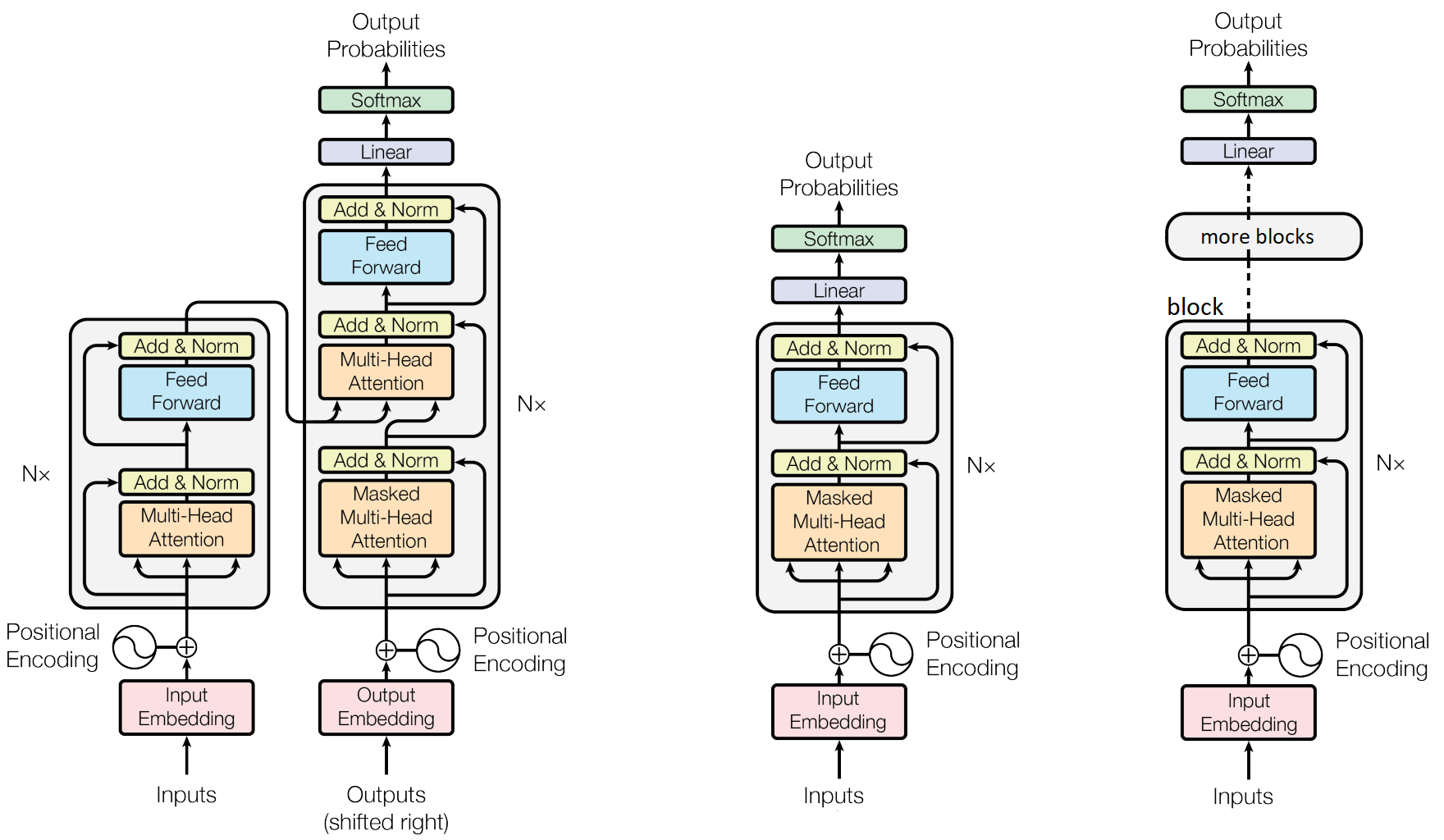
Left: the original transformer structure with an endocer and a decoder block. Middle: a single-block decoder-only model architecture. Right: the multi-block GPT decoder-only architecture, detailed here. Source: adapted from Attention is all you need.
Hyperparameters
The basic imports and the ML hyperparameters are:
import torch
import torch.nn as nn
import torch.nn.functional as F

# set the random seed, for reproducibility
torch.manual_seed(42)

# device: where to execute computation
device = torch.device("cuda" if torch.cuda.is_available() else "cpu")

# how often to do an evaluation step
eval_interval = 100

# number of training iterations
max_iters = 500

# optimizer's learning rate
learning_rate=1e-4

# minibatch size, how many inputs to 'pack' per iteration
batch_size = 3
and the ones specific to the GPT model are:
# block size is the maximum sequence length used as input.
# E.g. for block_size 4 and input ABCD, we have training samples A->B, AB->C, ABC->C, ABCD->E
block_size = 4

# size of the embeddings
n_embd = 16

# number of attention heads in Multi-Attention mechanism (the Nx in the GPT decoder diagram)
n_head = 6

# depth of the network as number of decoder blocks.
# Each block contains a normalization, an attention and a feed forward unit
n_layer = 6

# dropout rate (variable p) for dropout units
dropout = 0.2
As input dataset, we will use the tiny shakespeare text. First download it from a console:
$ wget https://raw.githubusercontent.com/karpathy/char-rnn/master/data/tinyshakespeare/input.txt
and then load it in python:
with open("input.txt") as f:
    text = f.read()
Tokenization
We need to create an embedding that maps input characters to a numerical representation of tokens. There are several possible tokenizers, the most simple being an embedding that maps characters to integers directly:
# collect sorted list of input characters and create
# string-to-int (stoi) and int-to-string (itos) representations:
chars = sorted(list(set(text)))
stoi = { ch:i for i,ch in enumerate(chars) }
itos = { i:ch for i,ch in enumerate(chars) }

# define encode and decode functions that convert strings to arrays of tokens and vice-versa
encode = lambda x: torch.tensor([stoi[ch] for ch in x], dtype=torch.long) #encode text to integers
decode = lambda x: ''.join([itos[i] for i in x]) #decode integers to text
vocab_size = len(stoi)
The vocabulary size vocab_size is simply the number of distinct tokens. In this case, 65 characters:
!$&',-.3:;?ABCDEFGHIJKLMNOPQRSTUVWXYZabcdefghijklmnopqrstuvwxyz
, where the first character is the line break character \n.
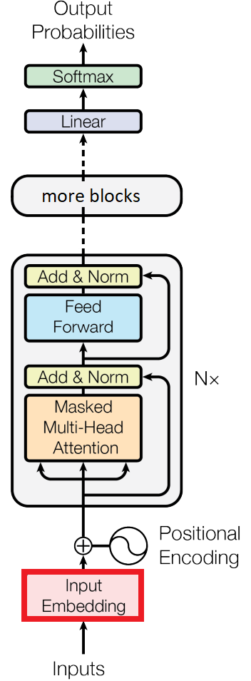
The embedding module in our model, emphasized in red.
For better context and smaller embeddings, we can pack several characters into each token, instead of encoding a character per token. As an example, we can encode entire words or subwords. Other possibilities of pre-existent tokenizers are google’s sentencepiece, the word or subword tokenizers by huggingface, or the Byte-Pair-Encoding (BPE) tiktoken used by OpenAI’s GPT:
import tiktoken
enc = tiktoken.encoding_for_model("gpt-4")
print(enc.n_vocab)
print(enc.encode("Hello world").tolist())
This would output vocabulary size of 100277 and [9906, 1917] and the encoding of "Hello World" as tokens and on itr original string representation.
Positional Encoddings
The Attention mechanism returns a set of vectors. Only by adding positional encondings to each token we can introduce the notion of sequence. In the original paper the authors use a positional embedding based on the \(sin\) and \(cos\) frequencies (see my previous Transformer post for details). For simplicity, we will use instead the Embedding function in pytorch.
token_embedding_table = nn.Embedding(vocab_size, n_embd)    # from tokens to embedding
position_embedding_table = nn.Embedding(block_size, n_embd) # from position to embedding
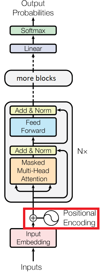
The positional encoding module in our model, emphasized in red.
Batching and dimensionality
First, we will do a train-validation data split of 90% and 10%:
data = encode(text)  #use any encoder here
n = int(0.9*len(data))
train_data, valid_data = data[:n], data[n:]
For this input: the full, train and validation datasets have 1115394, 1003854 and 111540 elements, respectively.
Batching in the attention mechanism is tricky. The model needs to accept a batch of several inputs, and each input will have a maximum size of block_size. For this to be possible, for a given input, the dataset includes all sequencies from size 1 to size block_size. For each input sequence from position 0 to t, the respective output is given by the element in positon t+1. This logic is better detailed by to following code:
def get_batch(source):
  """ get batch of size block_size from source """

  # generate `batch_size` random offsets on the data
  ix = torch.randint(len(source)-block_size, (batch_size,) )
  # collect `batch_size` subsequences of length `block_size` from source, as data and target
  x = torch.stack([source[i:i+block_size] for i in ix])
  # target is just x shifted right (ie the predicted token is the next in the sequence)
  y = torch.stack([source[i+1:i+1+block_size] for i in ix])
  return x.to(device), y.to(device)


# test get_batch()
xb, yb = get_batch(train_data)
print("input:\n",xb)
print("target:\n",yb)

for b in range(batch_size): #for every batches
  print(f"\n=== batch {b}:")
  for t in range(block_size): #for each sequence in block
    context = xb[b,:t+1]
    target = yb[b,t]
    print(f"for input {context.tolist()} target is {target.tolist()}")
this would output, for a block_size=4 and batch_size=3:
input:
 tensor([[45, 57,  1, 59],
        [ 1, 40, 43,  1],
        [39, 52, 42,  1]])

target:
 tensor([[57,  1, 59, 54],
        [40, 43,  1, 56],
        [52, 42,  1, 52]])

=== batch 0:
for input [45] target is 57
for input [45, 57] target is 1
for input [45, 57, 1] target is 59
for input [45, 57, 1, 59] target is 54

=== batch 1:
for input [1] target is 40
for input [1, 40] target is 43
for input [1, 40, 43] target is 1
for input [1, 40, 43, 1] target is 56

=== batch 2:
for input [39] target is 52
for input [39, 52] target is 42
for input [39, 52, 42] target is 1
for input [39, 52, 42, 1] target is 52
Multi-Head Masked Attention
The point of the attention mask is to define which elements are “visible” to other elements in the attention matrix, and by how much. A common example is to use a lower-diagonal attention matrix, that presents to each row (token), the current and previous tokens in the sentence. Each value in the attention matrix holds the “importance” that the column token infers – compared to all other columns of that row – when the row token needs to take a decision. Thus, the easiest implementation of an attention matrix is to simply add uniform weights across each row, so that all tokens have the same weight/importance:
Given a random input value x (shaped batch x time x channels):
B, T, C, = 4, 8, 2
x = torch.randn(B,T,C) #shape (B,T,C)
Note, for simplicity, we’ll use the following letters for the shapes of arrays:
- size
Cfor the embedding size of each token, defined by then_embedon top; - size
Bfor the batch size defined above bybatch_size; - size
Tfor the time dimension, or input sequence length, defined byblock_size.
We can compute an uniform attention matrix as:
#attention matrix (lower triangular), a mask used to only show previous items to predict next item
wei = torch.tril(torch.ones((T,T), dtype=torch.float32, device=device))
#normalize mask so that it sums to one. use keepdim to make broadcast operation work later
wei /= wei.sum(dim=1, keepdim=True)
or in an alternative notation (useful later):
tril = torch.tril(torch.ones(T,T))
wei = wei.masked_fill(tril==0, float('-inf'))
wei = F.softmax(wei, dim=-1) #equivalent to the normalization above
where both notations output as wei the following:
tensor([[1.0000, 0.0000, 0.0000, 0.0000, 0.0000, 0.0000, 0.0000, 0.0000],
        [0.5000, 0.5000, 0.0000, 0.0000, 0.0000, 0.0000, 0.0000, 0.0000],
        [0.3333, 0.3333, 0.3333, 0.0000, 0.0000, 0.0000, 0.0000, 0.0000],
        [0.2500, 0.2500, 0.2500, 0.2500, 0.0000, 0.0000, 0.0000, 0.0000],
        [0.2000, 0.2000, 0.2000, 0.2000, 0.2000, 0.0000, 0.0000, 0.0000],
        [0.1667, 0.1667, 0.1667, 0.1667, 0.1667, 0.1667, 0.0000, 0.0000],
        [0.1429, 0.1429, 0.1429, 0.1429, 0.1429, 0.1429, 0.1429, 0.0000],
        [0.1250, 0.1250, 0.1250, 0.1250, 0.1250, 0.1250, 0.1250, 0.1250]])
Again, the wei matrix indicates how much attention each token should give to itself and previous tokens, normalized to 1. In this case, it’s uniform.
We can do a dot-product of the input x by the attention wei and see the output of the attention head for the given x:
out = wei @ x # dot product shape: (B,T,T) @ (B,T,C) = (B,T,C) ie ([4, 8, 2])
Both x and out have dimensionlity [B, T, C] ie [4, 8, 2].
Now we move to the non-uniform attention matrix. The original paper formulates attention as:
\[MultiHead(Q, K, V ) = Concat(head_1, ..., head_h)W^O\] \[\text{where } head_i = Attention(QW^Q_i, KW^K_i, VW^V_i)\] \[\text{where } Attention(Q,K,V) = softmax \left( \frac{QK^T}{\sqrt{d_k}} \right) \, V\]
The multi-head (Nx) attention module in our model, emphasized in red.
Let’s start with the \(W^Q\), \(W^K\) and \(W^V\) matrices, computed as a simple projection (linear layer):
head_size=4
key   = nn.Linear(C, head_size, bias=False)
query = nn.Linear(C, head_size, bias=False)
value = nn.Linear(C, head_size, bias=False)
We can now compute the \(Attention(Q,K,V)\) as:
k = key(x) #shape (B,T, head_size)
q = query(x) #shape (B,T, head_size)
wei = q @ k.transpose(-2, -1) #shape (B,T, head_size) @ (B,head_size,T) = (B,T,T)
wei *= head_size**-0.5 #scale by sqrt(d_k) as per paper, so that variance of the wei is 1
We then adapt the (alternative) notation of the uniform attention above, and compute the output of the non-uniform attention matrix as:
tril = torch.tril(torch.ones(T,T))
wei = wei.masked_fill(tril==0, float('-inf')) #tokens only "talk" to previous tokens
wei = F.softmax(wei, dim=-1) #equivalent to the normalization above (-inf in upper diagonal will be 0)
v = value(x) # shape (B,T, head_size)
out = wei @ v # shape (B,T,T) @ (B,T,C) --> (B,T,C)
Note that out = wei @ x is the same inner dot-product of the previous items, but this time the attention weights are not uniform, they are learnt parameters and change per query and over time. And this is the main property and the main problem that the self-attention solves: non-uniform attention weights per query. This is different than the uniform attention matrix where weights were uniform across all previous tokens, i.e. aggregation was just a raw average of all tokens in the sequence. Here we aggregate them by a “value of importance” for each token.
Also, without the \(\sqrt{d_k}\) normalisation, we would have diffused values in wei, and it would approximate a one-hot vector. This normalization creates a more sparse wei vector.
This mechanism we coded is called self-attention because the \(K\), \(Q\) and \(V\) all come from the same input x. But attention is more general. x can be given by a data source, and \(K\) ,\(Q\) and \(V\) may come from different sources – this would be called cross attention.
As final remarks, note that elements across batches are always independent, i.e. no cross-batch attention. And in many cases, e.g. a string representation of chemical compounds, or sentiment analysis, there can be no attention mask (i.e. all tokens can attend to all tokens), or there’s a custom mask that fits the use case (e.g. main upper and lower diagonals to allow tokens to see their closest neighbour only). And here, we also don’t have any cross atttention between the encoder and decoder.
The decoder includes a multi-head attention, which is simply a concatenation of individual heads’ outputs. The Head and MultiHeadAttention modules can then be implemented as:
class Head(nn.Module):

  def __init__(self, head_size):
    super().__init__()
    self.key   = nn.Linear(n_embd, head_size, bias=False)
    self.query = nn.Linear(n_embd, head_size, bias=False)
    self.value = nn.Linear(n_embd, head_size, bias=False)
    self.register_buffer('tril', torch.tril(torch.ones(block_size, block_size)))
    self.dropout = nn.Dropout(dropout)
    #Note: this dropout randomly prevents some tokens from communicating with each other

  def forward(self, x):
    B,T,C = x.shape
    k = self.key(x) #shape (B,T, head_size)
    q = self.query(x) #shape (B,T, head_size)
    v = self.value(x) #shape (B,T, head_size)

    #compute self-attention scores
    wei = q @ k.transpose(-2, -1) #shape (B,T, head_size) @ (B,head_size,T) --> (B,T,T)
    wei *= C**-0.5 #scale by sqrt(d_k) as per paper, so that variance of the wei is 1
    wei = wei.masked_fill(self.tril[:T,:T]==0, float('-inf')) # (B,T,T)
    wei = F.softmax(wei, dim=-1) # (B, T, T)
    wei = self.dropout(wei)

    #perform weighted aggregation of values
    out = wei @ v # (B, T, T) @ (B, T, head_size) --> (B, T, head_size)
    return out
class MultiHeadAttention(nn.Module):
  """ Multi-head attention as a collection of heads with concatenated outputs."""
  def __init__(self, num_heads, head_size):
    super().__init__()
    self.heads = nn.ModuleList([Head(head_size) for _ in range(num_heads)])
    self.proj  = nn.Linear(head_size*num_heads, n_embd) # combine all head outputs
    self.dropout = nn.Dropout(dropout)

  def forward(self, x):
    out = torch.cat([head(x) for head in self.heads], dim=-1)
    out = self.proj(out)
    out = self.dropout(out)
    return out
Feed Forward Network
The Feed-forward network (FFN) in the decoder is simply a single-layer Deep Neural Network and is pretty straighforward to implement:
class FeedForward(nn.Module):
  """ the feed forward network (FFN) in the paper"""

  def __init__(self, n_embd):
    super().__init__()
    # Note: in the paper (section 3.3) we have d_{model}=512 and d_{ff}=2048.
    # Therefore the inner layer is 4 times the size of the embedding layer
    self.net = nn.Sequential(
        nn.Linear(n_embd, n_embd*4),
        nn.ReLU(),
        nn.Linear(n_embd*4, n_embd),
        nn.Dropout(dropout)
      )

  def forward(self, x):
    return self.net(x)

The feed forward network in our model, emphasized in red.
The GPT Block
We’ll call GPT block the sequence of a multi-head attention and a feedforward module. There are some subtle improvements we’d like to emphasize. Because the network can become too deep (and hard to train) for a high number of sequential blocks, we added skip connections to each block. Also, in the original paper, the layer normalization operation is applied after the attention and the feed-forward network, but before the skip connection. In modern days, it is common to apply it in the pre-norm formulation, where normalization is applied before the attention and the FFN. That’s also what we’ll do in the following code:
class Block(nn.Module):
  """ Transformer block: comunication (attention) followed by computation (FFN) """

  def __init__(self, n_embd, n_head):
    # n_embd: embedding dimension
    # n_heads : the number of heads we'd like to use
    super().__init__()
    head_size = n_embd // n_head
    self.sa = MultiHeadAttention(n_head, head_size)
    self.ffwd = FeedForward(n_embd)
    self.ln1 = nn.LayerNorm(n_embd)
    self.ln2 = nn.LayerNorm(n_embd)

  def forward(self, x):
    x = x + self.sa(self.ln1(x))
    x = x + self.ffwd(self.ln2(x))
    return x

The GPT block(s) in our model, emphasized in red.
Final Model
Putting it all together, our main model is wrapped as:
class GPTlite(nn.Module):

  def __init__(self, vocab_size):
    super().__init__()

    # vocabulary embedding and positional embedding
    self.token_embedding_table = nn.Embedding(vocab_size, n_embd)
    self.position_embedding_table = nn.Embedding(block_size, n_embd)

    #sequence of attention heads and feed forward layers
    self.blocks = nn.Sequential( *[Block(n_embd, n_head) for _ in range(n_layer)])

    #one layer normalization layer after transformer blocks
    #and one before linear layer that outputs the vocabulary
    self.ln = nn.LayerNorm(n_embd)
    self.lm_head = nn.Linear(n_embd, vocab_size, bias=False)


  def forward(self, idx):
    """ call the model with idx and targets (training) or without targets (generation)"""

    #idx and targets are both of shape (B,T)
    B, T = idx.shape
    tok_emb = self.token_embedding_table(idx) #shape (B,T,C)
    pos_emb = self.position_embedding_table(torch.arange(T, device=idx.device)) #shape (T,C)
    x = tok_emb + pos_emb #shape (B,T,C)
    x = self.blocks(x)
    x = self.ln(x)
    logits = self.lm_head(x) #shape (B,T,C)
    logits = torch.swapaxes(logits, 1, 2) #shape (B,C,T) to comply with CrossEntropyLoss
    return logits
and the inference (token generation) function is:
  def generate(self, idx, max_new_tokens):
    """ given a context idx, generate max_new_tokens tokens and append them to idx """
    for _ in range(max_new_tokens):
      idx_cond = idx[:, -block_size:] #we can never have any idx longer than block_size
      logits = self(idx_cond) #call fwd without targets
      logits = logits[:, :, -1] # take last token. from shape (B, C, T) to (B, C)
      #convert logits to probabilities
      probs = F.softmax(logits, dim=-1) # shape (B, C)
      #randomly sample the next tokens, 1 for each of the previous probability distributions
      #(one could take instead the argmax, but that would be deterministic and boring)
      idx_next = torch.multinomial(probs, num_samples=1) # shape (B, 1)
      #append next token ix to the solution sequence so far
      idx = torch.cat([idx, idx_next], dim=-1) # shape (B, T+1)
    return idx
Train loop
Now we can instantiate the model and copy it to the compute device:
m = GPTlite(vocab_size).to(device)
We then initialize the optimizer and perform the train loop:
# train the model
optimizer = torch.optim.Adam(m.parameters(), lr=learning_rate)
for steps in range(max_iters):
  idx, targets = get_batch(train_data)   #get a batch of training data
  logits = m(idx)   #forward pass
  loss = F.cross_entropy(logits, targets)
  loss.backward()   #backward pass
  optimizer.step()   #update parameters
  optimizer.zero_grad(set_to_none=True)  #sets to None instead of 0, to save memory

  #print progress
  if steps % 100 == 0: print(f"step {steps}, loss {loss.item():.2f}")

  @torch.no_grad()
  # eval loop: no backprop on this data, to avoid storing all intermediatte variables
  def eval_loss():
    idx, targets = get_batch(valid_data)   #get a batch of validation data
    logits = m(idx)   #forward pass
    loss = F.cross_entropy(logits, targets)
    print(f"step {steps}, eval loss {loss.item():.2f}")
    return loss

  if steps % eval_interval == 0: eval_loss().item()
Size matters
We will now test the model. We pass a single token (the \n character, encoded as token 0) to the model as initial character, and let it generate a sequence of 500 tokens:
#a 1x1 tensor with batch size 1 and sequence length 1 and starting value 0 (0 is the \n character)
idx = torch.zeros((1,1), dtype=torch.long, device=device)

# test the same generate() function, now with the trained model
print(decode(m.generate(idx, max_new_tokens=500).tolist()[0]))
and this will start blabbing some text, which looks a bit random for now:
IVINILCHIUKI noes hereseoke

PIV:
Ansto not 'dk thit, lighinglest in, the tole Himpams witecoond My me,
Cothe pill cthermandunes
The yould hankenou sonogher dovings age's eenat orshe:
And? Camer ou heithande, sonteas
Ans d th sonce;s ee e a
Bet n severe ay an kin nthely; wid, min. se garfitin d,
s I at nd d tlineay hanoro f;'s ikeff t maleanta t t'san bus weleng, c,
Ther coressoonerves se ivenind s,
An then, e g
Anand nvienowhin, an somend tisefffospup thid meewgonevand s,
pe
Anony a onaneyou ynuplot fouthaies angen hr imoupe?

E CAsinoveatot toooven
A cevet heplig tsest were sis d whelen fen CLUny cer:
Aid: a d?
UFrrand age thak?

CEDUKINIG m.
Hak's; te!
This is because for the sake of this tutorial, we used very small parameters for our GPT lite model. Better results can be achieved by increasing several of the parameters above, such as batch size, larger attention and more GPT blocks. As an example, if you try the following:
eval_interval = 100
max_iters = 5000
learning_rate=3e-4
batch_size = 128
block_size = 256
n_embd = 300
n_layer = 10
dropout = 0.2
You will get a significant performance improvement:
Pettience! if Tybalt ally kny to the waywards
That we renow't I have satic I fain.
Provotest the office Paul wains up the dudght.

And MOLEO:
Then me findy,
I do from the king him. How going in him.

TRANIO:
Good mind beherd at the world hold I pray
Toke you remect. If all my vernant youth I bear you
Dod forth.

DUKE VINCENTIO:
And ambibed, my lords I am not thence unnat;
Why, how said, too determoly fear is mercy,
But whether by my swalind
Tless and Rome: what guess the catter
Than thou not pro
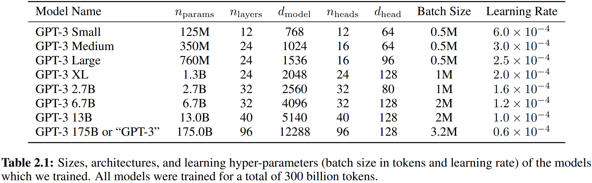
If you are interest on the real scale size, the paper Language Models are Few-Shot Learners provide us with several details related to the GPT-3:
Finetuning
The task that we detailed in this post is only the pre-training step of LLMs. This is the initial step that lets the model learn the text structure, grammar, syntax ans some knowledge of a general dataset. On top of that, it has been shown that a general model can then be finetuned to perform specific tasks with great performance by performing a follow up training on a smaller dataset of the related topic. See the paper Language Models are Few-Shot Learners for details on LLM specialization using few- and zero-shot setups.
However, for a better GPT-like model, there are several training steps that are considered:
- the pre-training step detailed above, the most important computationally as it takes most of the overall compute time.
- the supervised finetuning step that optimizes the model to a specific task. It is a training step analogous to the pre-training, with a human-supervised dataset (ie feedback loop) that is specific to the task we want to specialize the model on.
- the reward modelling aka Reinformcement Learning from Human Feedback (RLHF) step. The dataset is now a set of comparisons. We take the model and generate multiple completions. Then a human annotator ranks the completions. The inputs become triplets
prompt, completion, rewardfor each completion, and we perform supervised learning on the reward only (ie the models now have the capacity to output completions and the expected quality of each completion). This is then used to train the model. - the reinforcement learning step, where the reward is the value predicted from the model trained on the previous step:

source: video State of GPT
If you are interested in this particular GPT implementation or want to learn more about GPT in general, see the original tutorial video, OpenAI GPT-3 paper, and the nanoGPT repo. For an overview of the 4-step training process, see the video State of GPT and the paper Proximal Policy Optimization Algorithms.
For a faster memory-efficient implementation of an exact attention mechanism, see Flash Attention and Flash Attention 2.
All done! For the full python implementation of the code presented, see the repo GPT-lite repo.