Inference optimization (3): knowledge distillation, pruning and quantization
In the previous parts of this series, we sped up the inference of GPTlite with caching and batching (part 1) and faster attention (part 2). This post changes the model itself. The most effective way to make a model faster is to make it smaller. Distillation trains a small model to behave like a large one; pruning removes parts of a large model. The two are usually combined. Quantization keeps all the parts of the model, but stores its numbers with fewer bits. As before, all the code is in the repository of this post.
Knowledge distillation
Knowledge Distillation (KD) trains a student model from a teacher model. Information flows from a larger or pre-trained teacher to a smaller or untrained student, to make the student smaller and/or better than it would be if trained alone. The main rationale is that the soft labels produced by a trained network, i.e., its full output distribution, are a richer training signal than the user-provided hard labels.
As a quick example, take a two-label (dog, cat) classification task. An image of a cat that looks like a dog has the ground-truth label distribution [0,1]. A trained model, queried with the same image, outputs something like [0.4, 0.6]: it believes it is a cat, but it could also be a dog. The soft label [0.4, 0.6] carries more information than the hard label [0,1], and training a second model on such labels lets it use its capacity better, spending less of it on learning noise. In language modeling, the teacher’s distribution over the next token tells the student not only which token is right, but also which alternatives are plausible.
There are several categories of KD methods. The loss can match the soft labels of the student and the teacher, as in the example above, or intermediate representations such as feature maps. The student can be a scaled-down version of the teacher’s architecture, or a different one. In offline distillation, the teacher is trained first and then frozen while the student learns from it; in online distillation, both are trained simultaneously. We can use a single teacher or an ensemble of teachers.
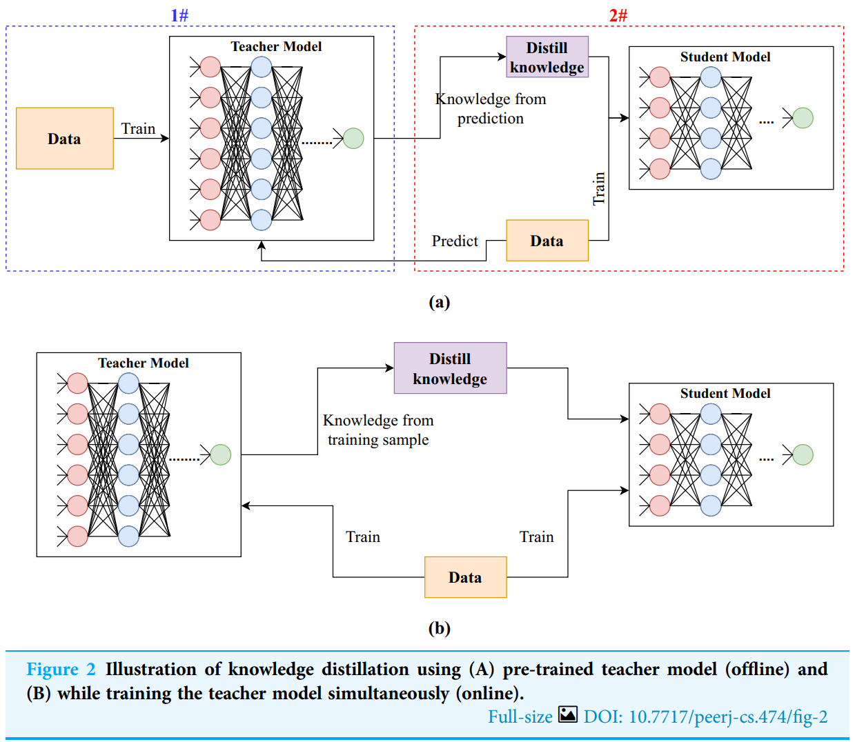
For details on the different methods, see Distilling the Knowledge in a Neural Network, Google, Knowledge distillation in deep learning and its applications, and Knowledge Distillation: A Survey.
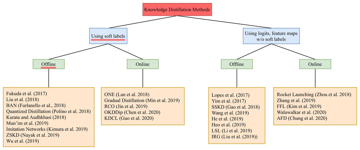
An illustration of the different categories of knowledge distillation methods, and of the branches within each category. In this section, we implement offline distillation using soft labels, underlined in red in the picture. Adapted from Knowledge distillation in deep learning and its applications.
Implementing offline distillation with soft labels
Our teacher is the pre-trained GPTlite, and our student is a smaller GPTlite with fewer layers and a smaller embedding. The teacher is frozen: it runs in evaluation mode (no dropout), and its forward pass runs inside torch.no_grad(), so that no computation graph or gradients are created for it. At every training step, both models process the same batch, and the student learns to match the teacher’s output distribution at every position of the sequence. We compute the teacher’s soft labels on the fly instead of storing them on disk: storing them takes batch size × sequence length × vocabulary size values per batch, and only pays off when the teacher is too large to run next to the student (in that case, one usually stores only the top-k logits, together with the inputs they belong to).
The loss is the Kullback-Leibler (KL) divergence between the teacher’s distribution \(p\) and the student’s distribution \(q\):
\[\begin{equation} \begin{split} D_{KL}(p \parallel q) & = H(p,q) - H(p) \\ & = - \sum_i p_i \log (q_i) + \sum_i p_i \log (p_i) \\ & = \sum_i p_i \log \frac{p_i}{q_i} \end{split} \end{equation}\]where \(H(p,q)\) is the cross entropy and \(H(p)\) the entropy of the teacher’s distribution. Since \(H(p)\) does not depend on the student, minimizing the KL divergence is equivalent to minimizing the cross entropy. The loss values differ, though: the KL divergence is zero when both distributions match, while the cross entropy equals the entropy of the target. This is why the cross entropy is the usual loss for hard labels, whose entropy is zero, and the KL divergence is used to compare two distributions. In PyTorch, F.kl_div expects the student’s log-probabilities as input. We also pass the teacher’s distribution as log-probabilities (log_target=True), which the documentation recommends to avoid numerical issues. We flatten the logits to shape (batch × sequence length, vocabulary size) and use reduction='batchmean', so that the loss is the mean KL divergence per token.
The temperature \(t\) controls how soft the distributions are. For logits \(z\), the softened output is:
\[y_i (x \mid t) = \frac{ \exp\frac{z_i(x)}{t} }{ \sum_j \, \exp\frac{z_j(x)}{t} }\]A temperature above 1 flattens the distribution and reveals the relative probabilities of the unlikely tokens, which carry most of the extra information. Since the gradients of the softened loss scale with \(1/t^2\), we multiply the loss by \(t^2\), as proposed by Hinton et al., so that the size of the gradients does not depend on the temperature. A common variant adds the regular cross entropy with the ground-truth labels, weighted by a factor \(\alpha\). There are also claims that the mean squared error between logits works better than the KL divergence (Kim et al.). For LLMs, recent methods also train the student on sequences it generated itself, scored by the teacher (on-policy distillation), which removes the mismatch between the sequences seen in training and in generation.
The following code implements the distillation of GPTlite into a smaller student. The full code is in main_distillation.py:
Show code
def distillation_loss(logits_student, logits_teacher, temperature):
  """ KL divergence between the softened teacher and student distributions, averaged per token, and
      scaled by temperature^2 so that the size of the gradients does not depend on the temperature """
  vocab_size = logits_student.size(-1)
  log_softmax_student = F.log_softmax(logits_student.reshape(-1, vocab_size)/temperature, dim=-1)   #log softmax of student model
  log_softmax_teacher = F.log_softmax(logits_teacher.reshape(-1, vocab_size)/temperature, dim=-1)   #log softmax of teacher model
  return F.kl_div(log_softmax_student, log_softmax_teacher, log_target=True, reduction='batchmean') * (temperature ** 2)

# the teacher: the pre-trained GPTlite, frozen in evaluation mode
n_layers, d_model, n_heads, d_head, batch_size, lr, seqlen, dropout_p = get_gptlite_model_parameters()
model_teacher = GPTlite(vocab_size, d_model, n_heads, d_head, n_layers, dropout_p, seqlen).to(device).eval()
model_teacher.load_state_dict(torch.load(GPTLITE_CKPT_PATH, map_location=device))

# the student: a smaller GPTlite
n_layers, d_model, n_heads, d_head, batch_size, lr, seqlen, dropout_p = get_gptlite_distilled_model_parameters()
model_student = GPTlite(vocab_size, d_model, n_heads, d_head, n_layers, dropout_p, seqlen).to(device)
optimizer = torch.optim.Adam(model_student.parameters(), lr=lr)

for step in range(1, train_iters+1):
  model_student.train()
  idx, _ = get_batch(train_data, batch_size=batch_size, seqlen=seqlen)   #get a batch of training data
  idx = idx.to(device) #move data to GPU
  logits_student = model_student(idx)   #forward pass
  with torch.no_grad():
    logits_teacher = model_teacher(idx)   #forward pass of the frozen teacher, without gradients
  loss = distillation_loss(logits_student, logits_teacher, temperature)  #compute KL divergence loss
  loss.backward()   #backward pass
  torch.nn.utils.clip_grad_norm_(model_student.parameters(), max_norm=1.0) # gradient clipping to avoid exploding gradients
  optimizer.step()   #update parameters
  optimizer.zero_grad(set_to_none=True)  #sets to None instead of 0, to save memory
The student is useful on its own, as a faster model, and as the draft model for speculative decoding - we will cover speculative decoding in a separate post.
Pruning
Pruning removes parts of a trained model. It is a hard problem, for three reasons: we must decide what to remove without trying every option; the parts of a network are coupled, so removing one forces changes elsewhere; and removing anything hurts accuracy, which must then be recovered. A fourth difficulty is turning the removal into actual speed.
What can be removed. Unstructured pruning removes individual weights by setting them to zero. Structured pruning removes whole structures, which shrinks the weight matrices. In GPTlite, a linear layer nn.Linear(d_in, d_out) stores a weight matrix of shape d_out × d_in, so:
- removing MLP neuron \(j\) removes row \(j\) (and bias \(j\)) of the first MLP layer, and column \(j\) of the second;
- removing attention head \(h\) removes its \(d_\text{head}\) rows from the query, key and value projections, and the corresponding \(d_\text{head}\) columns of the output projection;
- removing embedding channel \(c\) removes column \(c\) of the token and position embeddings, entry \(c\) of every LayerNorm, column \(c\) of every matrix that reads from the residual stream (query, key and value projections, first MLP layer and final output layer), and row \(c\) (and bias \(c\)) of every matrix that writes to it (attention output projection and second MLP layer). Every layer changes, which makes this the hardest and most impactful dimension;
- removing a transformer block deletes it entirely; thanks to the residual connections, the shapes of the other blocks stay valid.
Unstructured sparsity needs special hardware. A weight matrix with 50% of zeros scattered at random is still multiplied as a dense matrix by GPUs, so it saves no time, and saves memory only with a sparse storage format. The exception is NVIDIA’s 2:4 semi-structured sparsity (Mishra et al.): in every group of 4 consecutive weights, 2 are zero, and the sparse tensor cores of Ampere and newer GPUs skip them, doubling the peak throughput of those matrix multiplications. The end-to-end speedups are smaller, since attention, memory traffic and the other operations are not accelerated.
How to decide what to remove. Pruning methods estimate the importance of each weight or structure, usually on a small calibration dataset:
- magnitude: small weights matter less (simple, but crude);
- activations: a neuron, head or channel whose activations are small on average contributes little (used by Minitron, below);
- weights times activations: Wanda scores each weight by \(\lvert W_{ij} \rvert \cdot \lVert X_j \rVert_2\), its magnitude times the norm of its input feature, and prunes without any retraining;
- gradients: the first-order Taylor expansion \(\lvert w \cdot \partial L / \partial w \rvert\) estimates how much the loss increases when \(w\) is removed (LLM-Pruner, which also groups coupled structures and removes them together);
- second-order information: SparseGPT prunes and updates the remaining weights to compensate, one column at a time, using the inverse Hessian (the same idea as GPTQ). It prunes 175B-parameter models to 50-60% unstructured sparsity, or to 2:4 sparsity, in one shot;
- layer redundancy: ShortGPT removes the blocks whose output is most similar to their input (by cosine similarity), since they change the hidden state the least;
- learned masks: Sheared-LLaMA learns which heads, neurons, channels and layers to keep to reach a target architecture.
The Minitron recipe. NVIDIA’s Minitron combines structured pruning with distillation:
- compute the importance of heads, MLP neurons and embedding channels from their activations, and the importance of each layer from how much removing it hurts, on a small calibration set of about a thousand samples;
- prune the model to the target architecture;
- retrain the pruned model by distilling from the original one (the KL divergence on the logits, from the previous section), using a few percent of the original training tokens;
- repeat for smaller sizes.
Deriving 8B and 4B models from a 15B one this way required up to 40 times fewer training tokens than training them from scratch, and gave better accuracy. A follow-up on Llama 3.1 8B found that width pruning (heads, neurons and channels) preserves more accuracy, while depth pruning (whole blocks) gives larger speedups. The key insight is that a pruned teacher is a much better starting point for the student than a random initialization.
We apply this recipe to GPTlite, removing half of the attention heads and MLP neurons of every block in two ways: in one shot, followed by distillation, and iteratively, removing 10% at a time and distilling after each step, with the same total number of distillation steps. As a baseline, we distill into the same small architecture from a random initialization.
The following code implements the importance of heads and neurons, the structured pruning and the experiment. The full code is in main_pruning.py:
Show code
def compute_importance(model, data, n_batches, batch_size, seqlen):
  """ Importance of every attention head (norm of its output) and every MLP neuron (absolute value of its
      ReLU output), summed over a calibration set """
  heads = [torch.zeros(block.mha.n_heads, device=device) for block in model.blocks]
  neurons = [torch.zeros(block.ffwd.net[0].out_features, device=device) for block in model.blocks]
  def head_hook(i, H, D):  # the input of the output projection concatenates the outputs of all heads
    def hook(module, inputs):
      heads[i] += inputs[0].reshape(-1, H, D).norm(dim=-1).sum(dim=0)
    return hook
  def neuron_hook(i):  # the output of the ReLU holds the activations of the MLP neurons
    def hook(module, inputs, output):
      neurons[i] += output.reshape(-1, output.size(-1)).abs().sum(dim=0)
    return hook
  hooks = []
  for i, block in enumerate(model.blocks):
    hooks.append(block.mha.out_proj.register_forward_pre_hook(head_hook(i, block.mha.n_heads, block.mha.d_head)))
    hooks.append(block.ffwd.net[1].register_forward_hook(neuron_hook(i)))
  for _ in range(n_batches):
    x, _ = get_batch(data, batch_size=batch_size, seqlen=seqlen)
    model(x.to(device))
  for hook in hooks:
    hook.remove()
  return heads, neurons

def prune(model, heads, neurons, n_heads, n_neurons):
  """ Keeps the n_heads most important heads and the n_neurons most important MLP neurons of every block """
  for block, head_importance, neuron_importance in zip(model.blocks, heads, neurons):
    mha, D = block.mha, block.mha.d_head
    keep_heads = head_importance.topk(n_heads).indices.sort().values
    rows = (keep_heads[:, None] * D + torch.arange(D, device=device)).flatten()  # the d_head rows of each kept head
    mha.query_proj = prune_linear(mha.query_proj, rows=rows)
    mha.key_proj = prune_linear(mha.key_proj, rows=rows)
    mha.value_proj = prune_linear(mha.value_proj, rows=rows)
    mha.out_proj = prune_linear(mha.out_proj, columns=rows)
    mha.n_heads = n_heads
    keep_neurons = neuron_importance.topk(n_neurons).indices.sort().values
    block.ffwd.net[0] = prune_linear(block.ffwd.net[0], rows=keep_neurons)     # first MLP layer: one row per neuron
    block.ffwd.net[2] = prune_linear(block.ffwd.net[2], columns=keep_neurons)  # second MLP layer: one column per neuron
  return model

# the experiment: one-shot and iterative pruning, followed by distillation from the original model (teacher)
model = prune(copy.deepcopy(teacher), *importance(teacher), *target_size(keep_ratios[-1]))
distill(model, teacher, train_data, distill_iters, lr, batch_size, seqlen)

model = copy.deepcopy(teacher)
for ratio in keep_ratios:
  prune(model, *importance(model), *target_size(ratio))
  distill(model, teacher, train_data, distill_iters // len(keep_ratios), lr, batch_size, seqlen)
Quantization
Quantization stores numbers with fewer bits. Weights take less memory, fewer bytes are read at every decode step (which is what limits decode), and low-precision tensor cores perform more operations per second. The cost is a loss of precision, which must stay small enough not to hurt the quality of the model.
Number formats
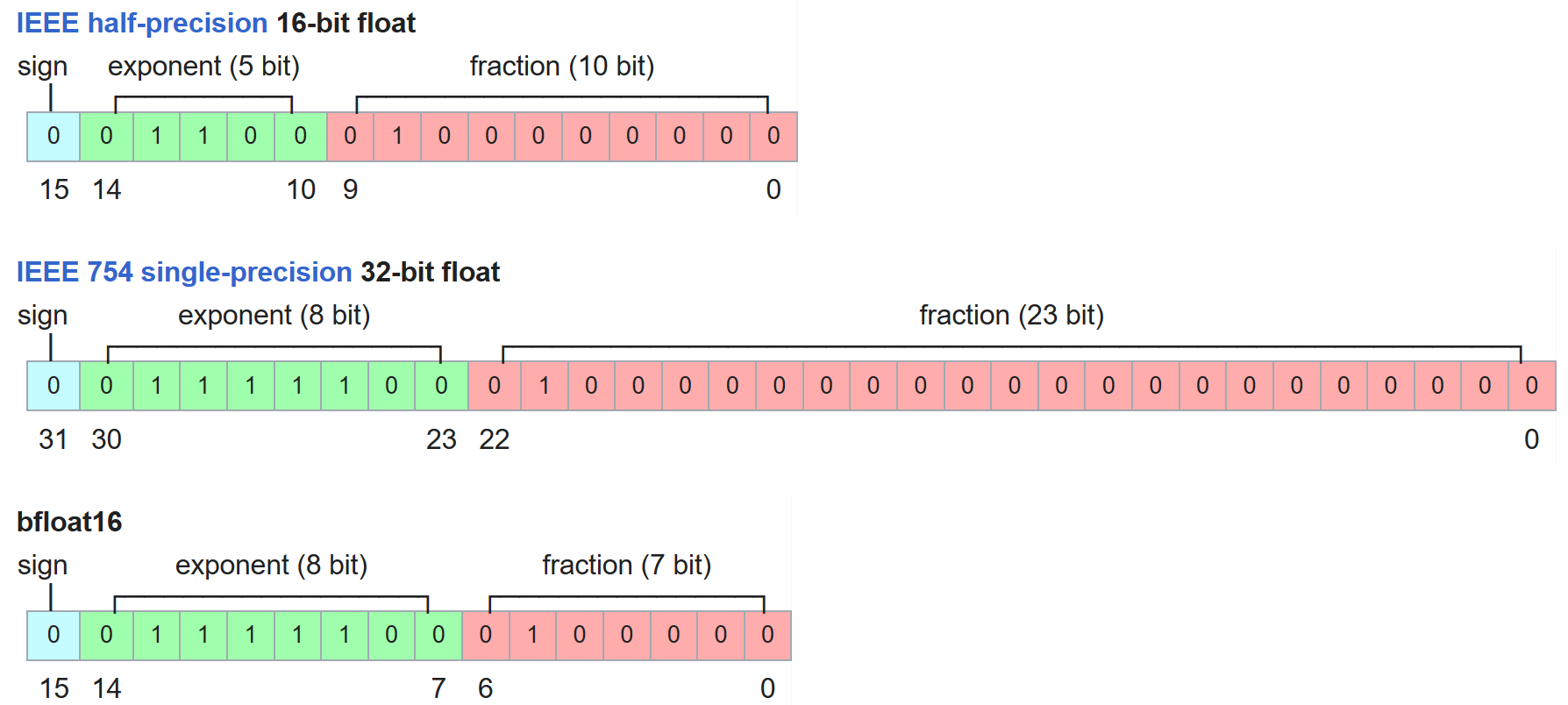
A floating point number has a sign bit, exponent bits that set its range, and mantissa (fraction) bits that set its precision. The picture below compares the three most common formats: FP32, FP16 and BF16. BF16 (brain floating point) keeps the 8 exponent bits of FP32 and only 7 mantissa bits, so it covers the same range as FP32 with the memory and speed of a 16-bit format. FP16 has more precision but a much smaller range (5 exponent bits), so large values can overflow. This is why BF16 is the default format of LLMs today.
Recent GPUs added smaller formats:
| Format | Bits | Sign / exponent / mantissa bits | Largest value | Typical use |
|---|---|---|---|---|
| FP32 | 32 | 1 / 8 / 23 | about 3.4 × 10³⁸ | reference precision |
| FP16 | 16 | 1 / 5 / 10 | 65,504 | weights and activations |
| BF16 | 16 | 1 / 8 / 7 | about 3.4 × 10³⁸ | default for LLM weights and activations |
| FP8 E4M3 | 8 | 1 / 4 / 3 | 448 | weights, activations and KV cache (Hopper, Ada and newer GPUs) |
| FP8 E5M2 | 8 | 1 / 5 / 2 | 57,344 | values that need more range than precision |
| FP4 E2M1 | 4 | 1 / 2 / 1 | 6 | weights and activations with micro-scaling (Blackwell GPUs) |
| INT8 | 8 | integers from -128 to 127 | 127 | weights, activations and KV cache |
| INT4 | 4 | integers from -8 to 7 | 7 | weights, with group-wise scales |
Four bits represent only 16 values: FP4 E2M1 can only represent \(\pm\{0, 0.5, 1, 1.5, 2, 3, 4, 6\}\). Such small formats only work with fine-grained scaling. In the micro-scaling (MX) formats, every block of 32 consecutive values shares an 8-bit power-of-two scale (MXFP8, MXFP6 and MXFP4), and NVIDIA’s NVFP4 uses blocks of 16 values with an FP8 scale, plus one FP32 scale per tensor. Blackwell tensor cores apply these scales in hardware. OpenAI’s gpt-oss models, for example, ship their mixture-of-experts weights in MXFP4.
How quantization works
To quantize a tensor \(x\) to \(b\)-bit integers, we choose a scale \(s\) (and optionally a zero-point \(z\)), then round and clip:
\[x_q = \text{clip}\left(\text{round}\left(\frac{x}{s}\right) + z, \; q_\text{min}, \; q_\text{max} \right), \quad\quad \hat{x} = s \, (x_q - z)\]where \(\hat{x}\) is the dequantized approximation of \(x\). In symmetric (absmax) quantization, \(z = 0\) and \(s = \max \lvert x \rvert / q_\text{max}\), e.g., with \(q_\text{max} = 127\) for INT8. Asymmetric quantization maps the range \([\min x, \max x]\) onto the full integer range, which fits skewed distributions better.
The granularity of the scales matters as much as the number of bits. A single scale per tensor is cheap but fragile. One scale per output channel (a row of the weight matrix), per group of, e.g., 128 consecutive weights, or per token for the activations, follows the data much more closely, at the cost of storing more scales. Group-wise scales are the standard for 4-bit weights.
The main enemy is outliers: a single large value stretches the scale, and all the small values collapse onto a few quantization levels. Weights are well-behaved and easy to quantize. Activations are not: LLM.int8() showed that large transformers develop a few outlier feature dimensions, with values much larger than the rest, that break naive 8-bit quantization of the activations.
Quantization can be applied after training with a small calibration dataset (post-training quantization, PTQ), which is fast and is what we do here, or simulated during training so that the model learns to tolerate it (quantization-aware training, QAT), which gives the best results at 4 bits and below. Finally, there are four things to quantize: the weights, the activations, the KV cache and the attention computation.
Weight-only quantization
Storing the weights in 4 or 8 bits while computing in 16 bits (e.g., W4A16: 4-bit weights, 16-bit activations) speeds up decode almost in proportion to the bytes saved, because decode is memory-bound: 4-bit weights are read four times faster than BF16 ones. The kernel must dequantize the weights on the fly, in registers, right before the multiplication; dequantizing the whole matrix to memory first would cancel the gain. Prefill, which is compute-bound, barely benefits.
Rounding each weight to the nearest level (round-to-nearest) works well at 8 bits, but loses too much accuracy at 4 bits. Two methods made 4-bit weights practical:
- GPTQ quantizes a weight matrix one column at a time and, after each column, updates the columns not yet quantized to compensate for the error just introduced. The update uses second-order information: the inverse of the Hessian \(H = 2XX^T\) of the layer’s reconstruction error, computed from calibration inputs \(X\). GPTQ quantizes 175B-parameter models to 3-4 bits in about four GPU hours.
- AWQ (Activation-aware Weight Quantization) observes that a small fraction of the weights matters much more than the rest: those that multiply large activations. Instead of keeping them in high precision, it multiplies the salient input channels of the weights by a factor before quantization (and divides the corresponding activations by the same factor, which can be folded into the previous operation), so that they are rounded more accurately. The factors are searched on calibration data.
Other common formats are NF4, from QLoRA, whose levels are placed for normally-distributed weights, and the GGUF formats of llama.cpp, for CPUs and edge devices.
To see how it works, we write our own quantizer: symmetric INT8 quantization with one scale per output channel, and INT4 quantization with one scale per group of 64 weights, packing two 4-bit weights per byte. It quantizes the linear layers of the transformer blocks of GPTlite, and we compare the memory, the time per token and the validation loss against the FP32 and BF16 models. With one scale per output channel, the INT8 layer can apply the scale after the matrix multiplication, while the INT4 layer must dequantize the weights first. In plain PyTorch, both convert the weights back to floating point in memory before each multiplication, which saves memory but not time: actual speedups require kernels that dequantize in registers, such as those of torchao or Marlin, or a compiler that fuses the conversion into the multiplication.
The following code implements our own weight-only INT8 and INT4 quantization of GPTlite. The full code is in main_quantization.py:
Show code
class QuantizedLinear(nn.Module):
  """ Linear layer with symmetric (absmax) weight-only quantization: INT8 with one scale per output channel,
      or INT4 with one scale per group of group_size consecutive weights of a row, packing two weights per byte.
      The weights are dequantized on the fly, and the computation runs in the precision of the input """

  def __init__(self, linear, bits, group_size=64):
    super().__init__()
    assert bits in (4, 8), "only 8 and 4 bits are supported"
    W = linear.weight.data  # [out_features, in_features]
    self.bits, (self.out_features, self.in_features) = bits, W.shape
    self.bias = None if linear.bias is None else nn.Parameter(linear.bias.data.clone(), requires_grad=False)
    q_max = 2 ** (bits - 1) - 1  # 127 for INT8, 7 for INT4
    if bits == 8:
      scale = W.abs().amax(dim=1, keepdim=True) / q_max  # [out_features, 1]
    else:
      self.group_size = group_size if self.in_features % group_size == 0 else self.in_features
      W = W.view(self.out_features, -1, self.group_size)   # [out_features, n_groups, group_size]
      scale = W.abs().amax(dim=2, keepdim=True) / q_max    # [out_features, n_groups, 1]
    scale = scale.clamp(min=1e-8)
    q = torch.clamp(torch.round(W / scale), -q_max - 1, q_max).to(torch.int8)
    if bits == 4:  # shift the values from [-8, 7] to [0, 15] and pack two of them per byte
      q = (q + 8).to(torch.uint8).view(self.out_features, -1)
      q = q[:, 0::2] | (q[:, 1::2] << 4)
    self.register_buffer('qweight', q)
    self.register_buffer('scale', scale)

  def dequantize(self):
    """ Weight matrix in the precision of the scales """
    if self.bits == 8:
      return self.qweight.to(self.scale.dtype) * self.scale
    low, high = (self.qweight & 0x0F).to(torch.int8) - 8, (self.qweight >> 4).to(torch.int8) - 8
    q = torch.stack([low, high], dim=-1).view(self.out_features, -1, self.group_size)  # unpack and interleave
    return (q.to(self.scale.dtype) * self.scale).view(self.out_features, self.in_features)

  def forward(self, x):
    if self.bits == 8:
      # with one scale per output channel, the scale can be applied after the matrix multiplication
      out = F.linear(x, self.qweight.to(x.dtype)) * self.scale.view(-1).to(x.dtype)
      return out if self.bias is None else out + self.bias
    return F.linear(x, self.dequantize().to(x.dtype), self.bias)

def quantize(model, bits, group_size=64):
  """ Replaces the linear layers of the transformer blocks by quantized ones. The embeddings and the
      output layer stay in full precision """
  linears = [(parent, name, child) for block in model.blocks for parent in block.modules()
             for name, child in parent.named_children() if isinstance(child, nn.Linear)]
  for parent, name, child in linears:
    setattr(parent, name, QuantizedLinear(child, bits, group_size))
  return model
Weight and activation quantization
To make the matrix multiplication itself faster, both of its inputs must be in low precision, so that the GPU can use its INT8, FP8 or FP4 tensor cores, which are 2 to 4 times faster than the BF16 ones. This also speeds up the compute-bound prefill and large-batch decode. The difficulty is the outliers of the activations:
- LLM.int8() keeps the few outlier feature dimensions in 16 bits and runs everything else in INT8.
- SmoothQuant moves the difficulty from the activations to the weights. Dividing the \(j\)-th channel of the activations by a factor \(s_j\), and multiplying the \(j\)-th input channel of the weights by the same factor, does not change the output of the layer but tames the outliers. With \(s_j = \max \lvert X_j \rvert^\alpha / \max \lvert W_j \rvert^{1-\alpha}\) and typically \(\alpha = 0.5\), both the weights and the activations become easy to quantize to INT8 (W8A8).
- FP8 weights and activations are the most common choice on Hopper and Blackwell GPUs: with per-channel or per-token scales, they are nearly lossless for most LLMs.
- Rotations (QuaRot, SpinQuant) multiply the weights and activations by orthogonal matrices, such as Hadamard matrices. Since \(RR^T = I\), the output does not change, but the rotation spreads each outlier across all channels. This makes 4-bit weights, activations and KV cache possible (W4A4KV4).
- FP4 (NVFP4 and MXFP4) on Blackwell GPUs uses the micro-scaled formats described above, for weights and activations.
KV cache quantization
At long contexts and large batches, the KV cache can be larger than the model weights. Storing it in FP8 or INT8 halves its size and the bytes read at each decode step, with almost no loss of quality; most serving engines enable it with a single configuration flag. More aggressive methods go down to 2 bits: KIVI quantizes the keys per channel, since their outliers live in fixed channels, and the values per token, and keeps the most recent tokens in full precision. Quantized attention kernels, such as SageAttention, apply the same ideas to the attention computation itself (see part 2).
Which one to use
A reasonable order: start in BF16; quantize the KV cache to FP8 for long contexts; use FP8 weights and activations on Hopper or newer GPUs; use 4-bit weights (AWQ or GPTQ) when memory is the constraint or the batch size is small; and use FP4 on Blackwell GPUs, ideally with a model trained or fine-tuned for it (QAT). Always measure the quality as well as the speed: the perplexity on held-out data, and the tasks you care about.