Distributed Matrix Transpose Algorithms
Matrix transpose is a problem of high importance, specially on fields such as large-scale algebraic resolutions and graph-based algorithms. The transpose of a graph provides the converse of the edge connectivity of a graph and the orthogonal view of its connectivity matrix. Although a tranpose of an algebraic table (or equivalently the connectivity matrix of a graph) may seem trivial when executed on a single compute node, it becomes a hard task when the dataset is distributed across multiple compute nodes.
This post details an efficient method to solve that problem, and shows how to implement it using the Message Passing Interface (MPI) runtime for distributed execution.
The basics
A graph \(G = (V, E)\) is a data structure consisting of a set of nodes or vertices \(V\), and a set of inter-node connections of edges \(E\). An edge \(\{i,j,e\} \subset \{\mathbb{N}, \mathbb{N}, T\}\) in \(E\) represents a connection between vertices \(i\) and \(j\) in \(V\) with edge information of type \(T\), and can be either ordered or unordered, depending on whether the graph is directed on undirected. A matrix \(M\) represents the connectivity \(E\) in \(G\), iff for all \(\{i,j,e\} \in E\), if \(G\) is ordered then \(M_{ij}=e\), and if is unordered then \(M_{ij} = M_{ji} = e\). Since \(M\) holds the possible connectivity between nodes in \(V\), then \(M\) is a square matrix of size \(|V| \times |V|\).
When a matrix is stored in a single compute node, the transpose is easy and follows the mathematical notation: a transpose of a matrix \(M\) is defined by \(M^T_{ij} = M_{ji}\), and holds an converse column-row cell placement of the initial matrix. The graph with connectivity described by a matrix \(M^T\) can be then described simply by \(G^{\star} = (V, E^{\star})\), where \(E^{\star} = \big\{ \{j,i,e\}\) for all \(\{i,j,e\} \in E \big\}\). In pratice, elements follow a row-column swap:
![]()
(image source: wikipedia)
Given a dense matrix representation of a graph connectivity \(E\), the algorithm to compute \(G^{\star}_{r} = (V_{r}, E^{\star}_{r})\) for every rank \(r\), requires only the computation of the matrix \(M^{T}_{r}\) for the connectivity \(E^{\star}_{r}\). Note that vertices information is local to a compute node, and they are still resident in the same memory location after transpose,
therefore the nodes information \(V\) is the same for \(G\) and \(G^{\star}\). The implementation of the distributed transpose is well known for a dense connectivity matrix, and available via the MPI_Alltoall collective call, that inputs (outputs) an array of elements, the size of the array, and datatype of the elements to be sent (received).
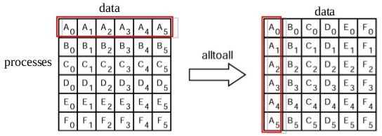
(image copyright: MPI Tutorial Shao-Ching Huang IDRE High Performance Computing Workshop 2013-02-13)</span>
For sparse matrices, the problem is not so trivial. A distributed memory data layout assumes that the vertices \(V\) are distributed across \(R\) compute nodes (ranks) and only rows local to each memory region are directly accessible to a rank. We will refer to \(G_{r} = (V_{r}, E_{r})\) as the subset of \(G\) that is stored in rank \(r\), with vertices \(V_{r}\) and edges \(E_{r}\). Each rank holds a disjoint subset of rows of the initial graph \(G\), such that cover ( \(\bigcup\limits_{r} G_{r} = G\)) and distinct (\(G_{r} \bigcap G_{s} = \emptyset, \forall r \neq s\)) properties hold. Ranks only hold information about outgoing connectivity (or from edges in this rank to other vertices), i.e. \(E_{r} = \Big\{ \{i,j,e\} \in E\) such that \(i \in V_r \Big\}\). Thus, the same cover and disjoint properties also hold for edges.
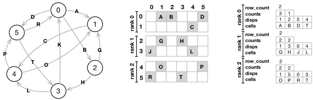
A common format utilised on the distributed storage of a sparse matrix is the Compressed Sparse Row (CSR) format, where each submatrix stored on a compute node is represented (serialized) as three arrays, representing (1) the number of populated columns per rows, (2) the id of each column populated, and (3) their respective values. For clarity, in the following picture we illustrate a sample graph with edges 0-5 and vertices A-P, its representative sparse matrix, and the CSR data structure on 3 ranks:
How to transpose it?
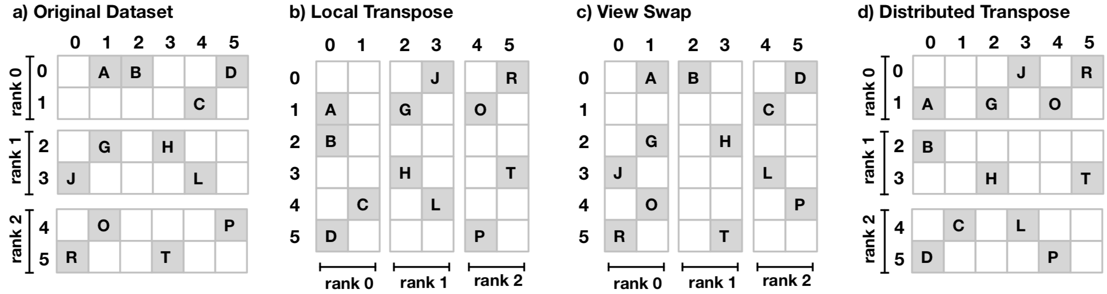
A small mental trick to understand this is to notice that a sparse matrix transpose is nothing more than a composition of two operations: a local matrix transpose and a view swap. So we can use these two operations and describe a distributed sparse matrix in four different data layouts, illustrated by:
We start the formulation of our problem resolution with the mathematical formalism underlying the distributed matrix transpose operations. A horizontal concatenation of two matrices \(M_{n \times m}\) and \(N_{n \times m'}\) is represented by \(M \| N\) and defined as the operation to join two sub-matrices horizontally into a matrix of dimensionality \({n \times (m+m')}\), such that:
\[(M \| N)_{i j} =\left\{ \begin{array}{@{}ll@{}} M_{i \,\, j} & \text{, if } j \leq m\\ N_{i \,\, j-m} & \text{, otherwise} \end{array}\right.\]Analogously, a vertical concatenation \(M_{n \times m} // N_{n' \times m}\) joins vertically two sub-matrices into a matrix of dimensionality \({(n+n') \times m}\), such that:
\[(M // N)_{i j} =\left\{ \begin{array}{@{}ll@{}} M_{i \,\, j} & \text{, if } i \leq n\\ N_{i-n \,\, j} & \text{, otherwise} \end{array}\right.\]We refer to a view as the perspective of data storage: a row view describes the matrix as the vertical concatenation of the subsets of rows stored on each rank. The column view represents the horizontal concatenation of subsets of columns on each rank. It follows that \((M \| N)^T = (N^T // M^T)\) and \((M // N)^T = (N^T \| M^T)\), as both concatenations provide the same dataset described by two alternative views, and the transpose of a concatenated dataset yields the orthogonally-concatenated dataset.
The local transpose of a matrix \(M\) represented by the concatenation of \(R\) submatrices in either view, is defined by the concatenation of the transpose of the individual matrices in the orthogonal view:
\[LocalTranspose(M)_{i j} =\left\{ \begin{array}{@{}ll@{}} \big( M^T_1 \| M^T_2 \| ... \| M^T_R \big)_{j i}& \text{, if } M \text{ is in row view }\\ \big( M^T_1 // M^T_2 // ... // M^T_R \big)_{j i}& \text{, otherwise} \end{array}\right.\]It is relevant to emphasize that the operation yields a transposed version of the original rank matrices that formed the initial dataset, thus no communication between ranks is necessary as the data \(M_r\) of every rank is locally transposed into \(M^T_r\). Moreover, it is an involutory function as \((LocalTranspose \cdot LocalTranspose) (M) = M\).
The view swap of a distributed matrix that alternates between a data representation on a view and its orthogonal (from row- to column-accessible and vice-versa), while maintaining the same matrix contents is defined by:
\[ViewSwap(M)_{i j} =\left\{ \begin{array}{@{}ll@{}} \big( M_1 \| M_2 \| ... \| M_R \big)_{i j}& \text{, if } M \text{ is in row view}\\ \big( M_1 // M_2 // ... // M_R \big)_{i j}& \text{, otherwise} \end{array}\right.\]At the level of a rank, the matrix data layout after a view swap is unknown until the swap is performed, as ranks do not hold information about the matrix structure across other ranks. Therefore, a communication step is required to be executed beforehand, in order to gather the number of rows held by individual ranks, and compute the row intervals on every other rank \(r\) as \(\big[ \sum^{r-1}_{r=1} |V_r|, \,\, \sum^{r}_{r=1} |V_r| \big)\).
This information is required for the correct matching of column/row id to target rank, used in the sparse transpose steps that follow. The view swap algorithm follows then in two communication steps. The first step performs a dense matrix transpose to send/receive the number of elements to/from other ranks. The second step performs a selective scatter-gather (MPI_Alltoallv) that delievers the elements to the final rank.
![]()
A memory realignment based on colum id and row id leads to the final distributed matrix dataset. To finalize, the view swap method is also an involutory function, as each view swap performs two involutory transpose operations, and two consecutive view swaps yield the initial dataset.
The full transpose algorithm performs only three collective communication calls, requiring an MPI_Allgather to compute the row offsets of ranks, and one MPI_Alltoall and MPI_Alltoallv for the metadata and cell values transpose in the view swaep. Moreover, the involutory property of our transpose method is a property of high importance, as it guarantees that distributed transpose can be validly executed any number of times, while respecting the data integrity of a CSR-based graph problem representation.
Algorithmic verification
Is this algorithm guaranteed to work independently of the dataset? We will show that it is indeed mathematically sound.
The distributed sparse transpose is defined by a composition of the local transpose and view swap methods. We have shown that both the local transpose and the view swap are XCSR compatible. We will show the distributed sparse transpose is also mathematically sound. Take a matrix \(M\) in row view, represented by the vertical concatenation of partial matrices \(M_1 // M_2 // ... // M_R\). A local transpose of \(M\) leads to \(M^T_{i j} = ( M^T_1 \| M^T_2 \| ... \| M^T_R)_{ji}\). Applying a view swap, we have \(M^T_{i j} = ( M^T_1 // M^T_2 // ... // N^T_R)_{ji}\), which is the definition of the distributed transpose of \(M\) in the original view. In brief, it follows that \(Transpose (M) = (LocalTranspose \cdot ViewSwap) (M)\).
The verification of the commuted involutory functions with \(Transpose (M) = (ViewSwap \cdot LocalTranspose) (M)\) also holds: a view swap over the original dataset leads to \(M_{i j} = ( M_1 // M_2 // ... // M_R)_{i j}\). The composition of a local transpose yields the final result \(M^T_{i j} = ( M^T_1 // M^T_2 // ... // N^T_R)_{ji}\). As \(Transpose\) is a composition of two involutory functions, and because both functions commute i.e. \((ViewSwap \cdot LocalTranspose) = (LocalTranspose \cdot ViewSwap)\), then \(Transpose\) is by definition involutory (Elements of operator theory, Kubrusly and Carlos S, Springer 2011)
Higher Cardinality Matrices
Single edges between pairs of nodes is a property that is often unavailable in real life situations. Take as an example the matrix representing information about common interests between pairs of users in a social network connectivity: some pairs of users may be connected by hundreds of common interests, while others may be connected by barely any interests in common; or an URLs cross-referral map, where one may be required to store not only the number of hyperlinks between pages, but also additional information about every link. How to implement the new transpose?
We start by the definition of a data format that can allocate high cardinality elements per graph node. We will call it the extended CSR, or XCSR for shortness, and we define it as the previous CSR data structure with an added dimensionaly to include number of elements per matrix cell (or edges between pairs of nodes). The layout is as follows:

The transpose algorithm follows then in three steps. First, each compute node (rank) collects the metadata of its own sub-matrix, composed by the set of triplets on the form [ row id, column id, number of elements], indicating the row colum and dimensionionality of each cell. Then they perform a local transpose of their own data, by reordering their triplets by colum and row id. This sequence illustrates the first step:
![]()
The second step starts the view swap method. All ranks pack and exchange (i.e. an all-to-all communication) the set of triplets to the correct recipient of the cell in the final tranposed matrix. In practice, the previous local transpose operation already sorted each sub-matrix by columns (i.e by rows of the final transposed dataset), therefore the triplets are already grouped by destination rank. More importantly: the matrix composed of all triplets across all ranks is a distributed matrix of fixed element size per cell (a tuplet of fixed size). Therefore, to perform this exchange we execute the same distributed transpose that we presented above in section How to Transpose it?. After the exchange, all ranks will hold the triplets of the metadata (but not the data yet) of the final matrix structure:
![]()
Finally, the view swap is terminated by communicating the data, based on the metadata of the transposed matrix. At first, each rank counts the number of elements to be received. The matrix of distributed counts of all elements to be sent and received per rank is a dense matrix that can be transposed easily (MPI_Alltoall). Those counts will then be used to allocate the buffers for the incoming data and perform and MPI_Alltoallv to send/deliver the elements of the final matrix across all compute nodes. Upon completion, we sort the (previously column-oriented) elements by row and column, and we reach our final dataset:
![]()
To finalize, the full transpose algorithm requires five collective communication calls, performing an MPI_Allgather to compute the row offsets of ranks, two MPI_Alltoall and two MPI_Alltoallv for the metadata and cell values transpose. Moreover, the general applicability of the XCSR and the involutory property of our transpose method, are two properties of high importance as they guarantee that distributed transpose can be validly executed any number of times, while respecting the data integrity of a XCSR-based graph problem representation.
Further details
For more details, implementation and benchmark information, read the original publication (preprint) or download the source code.