Deep Neural Networks, Backpropagation and Optimization
In 1958, Frank Rosenblatt described the perceptron, an artificial neuron that learns to separate two classes with a linear boundary. In 1969, the book Perceptrons by Marvin Minsky and Seymour Papert showed that such a neuron cannot learn a function as simple as the exclusive or (XOR) of two binary inputs. No line separates the inputs \((0, 1)\) and \((1, 0)\), of output 1, from \((0, 0)\) and \((1, 1)\), of output 0. Networks with several layers of such neurons can learn XOR and much more complex functions. In 1986, the paper Learning representations by back-propagating errors, by David Rumelhart, Geoffrey Hinton and Ronald Williams, showed how to train them with gradient descent, by propagating the errors backwards from the output layer to the first one.
Deep Neural Networks (also known as Multi-Layer Perceptrons) are universal approximators, i.e. they can approximate any continuous function on a closed and bounded domain, even with a single hidden layer, given enough neurons. They are the most important and relevant ML tool in the field of supervised learning, as they are part of the models used for most supervised tasks. This post covers their structure, the loss functions that measure their error, the backpropagation algorithm that computes the gradients of the loss, with its implementation in NumPy and with automatic differentiation, and the optimizers that update their parameters, with a training loop. Dropout, convolutional networks, skip connections and embeddings follow in the post Dropout, CNNs, Skip Connections and Embeddings.
Feedforward Networks and Activation Functions
The structure of a basic NN is the following: one input layer of size \(D\), \(L\) hidden layers of size \(K\), and one output layer. It is a feedforward network: the computation performed by the network starts with the input from the left and flows to the right, with no feedback loop. It can be used for regression (when the output is a real value) and for classification (when the output is the class). The following picture illustrates a network with one hidden layer, where each node is connected to every node of the next layer, i.e. a fully connected network:
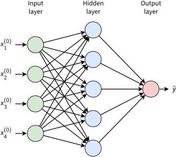
A fully connected feedforward network with an input layer of size \(D = 4\), one hidden layer of size \(K = 5\) and one output \(\hat{y}\). Adapted from: Machine Learning course CS-433 lecture notes, M. Jaggi, EPFL
Input and output layers work similarly to any previous regression method. Hidden layers are different. The output at node \(j\) in hidden layer \(l\) is given by:
\[x_j^{(l)} = \phi \left( \sum_i w_{i,j}^{(l)} x_i^{(l-1)} + b_j^{(l)} \right)\]where \(w_{i,j}^{(l)}\) is the weight of the connection from node \(i\) of layer \(l-1\) to node \(j\) of layer \(l\), and \(b_j^{(l)}\) is the bias term, trained like any other weight. Note that, to compute the output, each neuron first computes the weighted sum of its inputs and then applies an activation function \(\phi\) to this sum. The activation function must be non-linear, otherwise the whole network would be equivalent to a single linear layer. The function implemented by each layer can equally be described in matrix form:
\[x^{(l)} = f^{(l)} (x^{(l-1)}) = \phi ((W^{(l)})^T x^{(l-1)}+b^{(l)})\]where \(W^{(l)}\) is the matrix of the weights \(w_{i,j}^{(l)}\) of layer \(l\), \(b^{(l)}\) is the vector of its biases, \(\phi\) is applied to each entry, and \(f^{(l)}\) is the function implemented by the layer. Some popular choices of activation functions are:
- sigmoid function: \(\phi(x) = \frac{1}{1+e^{-x}}\), positive and bounded;
- tanh: \(\phi(x) = \frac{e^x - e^{-x}}{e^x+e^{-x}}\), balanced (positive and negative) and bounded;
- Rectified Linear Unit – ReLU: \(\phi(x) = [x]_+ = \max\{0,x\}\), always non-negative and unbounded; often used as it is computationally cheap and helps fight the issue of vanishing gradients in DNNs, as the positive output region does not have a small derivative;
- Leaky ReLU: \(\phi(x) = \max \{\alpha x,x\}\), with \(0 < \alpha < 1\). Fixes the dying ReLU problem of non-leaky rectified linear units;
- In brief, if the dot product of the input to a ReLU with its weights is negative, the output is 0. The gradient of \(\max\{ 0,x \}\) is \(0\) when the output is \(0\). If for any reason the output is consistently \(0\) (for example, if the ReLU has a large negative bias), then the gradient will be consistently 0. The error signal backpropagated from later layers gets multiplied by this 0, so no error signal ever passes to earlier layers. The ReLU has died. With leaky ReLUs, the gradient is never 0, and this problem is avoided.
In practice, ReLU and its variants are the default choice for hidden layers, while the sigmoid and tanh are used where a bounded output is needed, e.g. a probability at the output of a binary classifier. The following picture shows these functions and their derivatives:
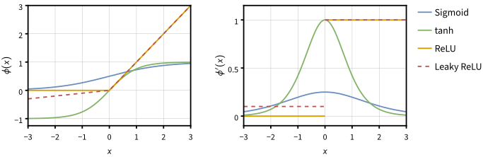
The sigmoid, tanh, ReLU and Leaky ReLU (with \(\alpha = 0.1\)) activation functions (left) and their derivatives (right). The derivatives of the sigmoid and tanh vanish for large \(\vert x \vert\), while the derivative of ReLU is 1 for every positive input and 0 for every negative input.
As an example, a network with two inputs, one hidden layer of two ReLU neurons and one output with no activation function computes the XOR that a single perceptron cannot learn. With the weights given in the Deep Learning book (section 6.1), the hidden layer computes \(x_1^{(1)} = \max\{0, x_1^{(0)} + x_2^{(0)}\}\) and \(x_2^{(1)} = \max\{0, x_1^{(0)} + x_2^{(0)} - 1\}\), and the output is \(\hat{y} = x_1^{(1)} - 2 x_2^{(1)}\). The four inputs \((0, 0)\), \((0, 1)\), \((1, 0)\) and \((1, 1)\) give the hidden outputs \((0, 0)\), \((1, 0)\), \((1, 0)\) and \((2, 1)\), and the outputs 0, 1, 1 and 0. The hidden layer maps the two inputs of output 1 to the same point, \((1, 0)\), where a linear output layer can separate them from the other two.
Without the ReLU, the same weights compute the linear function \(\hat{y} = 2 - x_1^{(0)} - x_2^{(0)}\), whose outputs 2, 1, 1 and 0 are not XOR: the non-linearity is what lets the hidden layer reshape its inputs. Here, the 6 weights and 3 biases of the network were set by hand. A network of millions of parameters learns them from data with gradient descent, which needs the derivative of the loss with respect to every parameter: this is the job of backpropagation.
Loss Functions
The loss function measures the error of the outputs of the network, and its choice depends on the task. Regression tasks mostly use the mean squared error (MSE), presented in the post on linear regression, with no activation function at the output layer, and classification tasks use the cross-entropy, which the post Statistics for ML relates to information theory.
With one-hot labels, the cross-entropy is equivalent to the negative log-likelihood (of the softmax, when the output of the model is not a distribution). However, to avoid numerical instabilities and overflows, implementations compute it directly from the output of the model, with the log-sum-exp trick. For the outputs (logits) \(a_1, ..., a_C\) of the model, the loss of a sample of class \(c\) is \(-\log \text{softmax}(a)_c = -a_c + a_{\max} + \log \sum_{j=1}^C \exp(a_j - a_{\max})\), where \(a_{\max} = \max_j a_j\), so that no exponential overflows. Most classification tasks use the binary or multi-class cross-entropy loss functions:
- binary: \(H(p) = -(y \log p(x) + (1-y) \log (1-p(x)))\), where \(p(x)\) is the predicted probability that the input \(x\) is of class 1, i.e. it simplifies to \(-\log p(x)\) for true label \(y=1\), and to \(-\log (1-p(x))\) for true label \(y=0\);
- multi-class: \(H(q,p) = -\sum_{c=1}^{C} q_c \log p_c\), over the \(C\) classes, for the true distribution \(q\) and the predicted distribution \(p\). With a one-hot label, only the term of the true class remains.
As an example, a prediction of 0.9 for the true class costs \(-\log 0.9 = 0.105\), while a prediction of 0.1 costs \(-\log 0.1 = 2.303\), 22 times more: the cross-entropy penalizes confident mistakes heavily.
The losses of other tasks, such as learning embeddings, labeling sequences and segmenting images, are presented in the post Dropout, CNNs, Skip Connections and Embeddings.
Backpropagation
Similarly to previous regression use cases, the loss of the system needs to be minimized, using e.g. Stochastic Gradient Descent. As always with gradient descent, the algorithm computes the gradient of the cost function for a particular input sample (with respect to all weights and bias terms), and takes a small step in the direction opposite to this gradient. The size of the step is set by the learning rate \(\eta\). Computing the derivative with respect to a particular parameter is an application of the chain rule of calculus. The cost function for the squared loss over \(N\) samples is written as:
\[\mathcal{L} = \frac{1}{N} \sum_{n=1}^N ( y_n - f^{(L+1)} \circ ... \circ f^{(2)} \circ f^{(1)} (x_n^{(0)}) ) ^2\]As the network is the composition of its layers, the chain rule gives the derivative of the loss with respect to the parameters \(\theta^{(l)}\) of each layer \(l\), its weights and biases, as a product of the derivatives of the layers after it:
\[\begin{align*} \frac{\partial \mathcal{L}}{\partial \theta^{(L+1)}} & = \frac{\partial \mathcal{L}}{\partial x^{(L+1)}} {\color{#0000FF} \frac{\partial x^{(L+1)}}{\partial \theta^{(L+1)}}} \\ \frac{\partial \mathcal{L}}{\partial \theta^{(L)}} & = \frac{\partial \mathcal{L}}{\partial x^{(L+1)}} \boxed{ {\color{#FF7300} \frac{\partial x^{(L+1)}}{\partial x^{(L)}}} {\color{#0000FF} \frac{\partial x^{(L)}}{\partial \theta^{(L)}}} } \\ \frac{\partial \mathcal{L}}{\partial \theta^{(L-1)}} & = \frac{\partial \mathcal{L}}{\partial x^{(L+1)}} {\color{#FF7300} \frac{\partial x^{(L+1)}}{\partial x^{(L)}}} \boxed{ {\color{#FF7300} \frac{\partial x^{(L)}}{\partial x^{(L-1)}}} {\color{#0000FF} \frac{\partial x^{(L-1)}}{\partial \theta^{(L-1)}}} } \\ \frac{\partial \mathcal{L}}{\partial \theta^{(l)}} & = \frac{\partial \mathcal{L}}{\partial x^{(L+1)}} {\color{#FF7300} \frac{\partial x^{(L+1)}}{\partial x^{(L)}}} \cdots \boxed{ {\color{#FF7300} \frac{\partial x^{(l+1)}}{\partial x^{(l)}}} {\color{#0000FF} \frac{\partial x^{(l)}}{\partial \theta^{(l)}}} } \end{align*}\]where the orange terms are partial derivatives of a layer with respect to its input, and the blue terms are partial derivatives of a layer with respect to its parameters. The boxed terms are the only new terms of each line; the rest is reused from the line above.
Since in general there are many parameters, it would not be efficient to do this for each parameter individually. As an example, estimating the gradient with finite differences takes one extra forward pass per parameter, i.e. a million forward passes for a network of a million parameters. However, the backpropagation algorithm does it more efficiently, as it computes the derivatives of all parameters with one forward and one backward pass through the network. The aim is to compute, for the loss \(\mathcal{L}_n\) of a sample \(n\):
\[\frac{\partial \mathcal{L}_n}{\partial w_{i,j}^{(l)}}, l=1, ..., L+1 \text {, and } \frac{\partial \mathcal{L}_n}{\partial b_{j}^{(l)}}, l=1, ..., L+1 \label{eq_gradient}\]For simplicity, the total input computed at the \(l\)-th layer, before the activation function, is represented as:
\[z^{(l)} = (W^{(l)})^T x^{(l-1)}+b^{(l)} . \label{eq_z}\]These quantities are easy to compute by a forward pass in the network, starting at \(x^{(0)} = x_n\) and then applying this recursion for \(l=1,...,L+1\).
Now, consider the derivative of the loss with respect to the total input of node \(j\) of layer \(l\), often called the error of the node:
\[\delta_j^{(l)} = \frac{\partial \mathcal{L}_n}{\partial z_j^{(l)}}. \label{eq_delta}\]These quantities are easier to compute with a backward pass, from the output layer to the first one, as the errors of each layer follow from those of the next layer:
\[\begin{align*} \delta_j^{(l)} = & \frac{\partial \mathcal{L}_n}{\partial z_j^{(l)}} \\ = & \sum_k \frac{\partial \mathcal{L}_n}{\partial z_k^{(l+1)}} \frac{\partial z_k^{(l+1)}}{\partial z_j^{(l)}} \\ = & \sum_k \delta_k^{(l+1)} \frac{\partial \left[ (W^{(l+1)})^T x^{(l)}+b^{(l+1)} \right]_k}{\partial z_j^{(l)}} \\ = & \sum_k \delta_k^{(l+1)} W_{j,k}^{(l+1)} \frac{\partial x_j^{(l)}}{\partial z_j^{(l)}} \\ = & \sum_k \delta_k^{(l+1)} W_{j,k}^{(l+1)} \phi '(z_j^{(l)}) \end{align*}\]The chain rule is used in the second equality, and, in the fourth, the fact that \(x_j^{(l)}\) is the only entry of \(x^{(l)}\) that depends on \(z_j^{(l)}\). The recursion starts at the output layer, where \(\delta^{(L+1)}\) follows from the derivative of the loss. For the squared loss of a sample, \(\mathcal{L}_n = (y_n - x^{(L+1)})^2\), and an output layer with no activation function, i.e. \(x^{(L+1)} = z^{(L+1)}\), it is given by \(\delta^{(L+1)} = -2 (y_n - x^{(L+1)})\).
Going back to equation \ref{eq_gradient}:
\[\frac{\partial \mathcal{L}_n}{\partial w_{i,j}^{(l)}} = \sum_k \frac{\partial \mathcal{L}_n}{\partial z_k^{(l)}} \frac{\partial z_k^{(l)}}{\partial w_{i,j}^{(l)}} = \delta_j^{(l)} x_i^{(l-1)} \label{eq_w}\]Here, the derivation uses the chain rule, the definition of \(\delta\) in equation \ref{eq_delta}, and the partial derivative of equation \ref{eq_z} with respect to \(w\), which is zero for \(k \neq j\). In a similar manner:
\[\frac{\partial \mathcal{L}_n}{\partial b_{j}^{(l)}} = \sum_k \frac{\partial \mathcal{L}_n}{\partial z_k^{(l)}} \frac{\partial z_k^{(l)}}{\partial b_{j}^{(l)}} = \delta_j^{(l)} \cdot 1 = \delta_j^{(l)} \label{eq_b}\]The complete backpropagation algorithm is then summarized as:
- Forward pass: set \(x^{(0)} = x_n\). Compute \(z^{(l)}\) for \(l=1,...,L+1\);
- Backward pass: set \(\delta ^{(L+1)}\) using the appropriate loss and activation function. Compute \(\delta ^{(l)}\) for \(l = L, ..., 1\);
- Final computation: for all parameters, compute \(\frac{\partial \mathcal{L}_n}{\partial w_{i,j}^{(l)}}\) (eq. \ref{eq_w}) and \(\frac{\partial \mathcal{L}_n}{\partial b_{j}^{(l)}}\) (eq. \ref{eq_b}).
As an example, consider a network with one neuron per layer, so that the indices \(i\) and \(j\) are dropped. Its input is \(x^{(0)} = x_n = 2\), its hidden neuron has the weight \(w^{(1)} = 1\) and a ReLU activation, and its output has the weight \(w^{(2)} = 0.5\) and no activation function. The biases are zero, and the target is \(y_n = 3\). The three steps of the algorithm give:
- Forward pass: \(z^{(1)} = 1 \times 2 = 2\), \(x^{(1)} = \max\{0, 2\} = 2\) and \(x^{(2)} = z^{(2)} = 0.5 \times 2 = 1\), so the loss is \((3 - 1)^2 = 4\);
- Backward pass: \(\delta^{(2)} = -2(3 - 1) = -4\), and \(\delta^{(1)} = \delta^{(2)} w^{(2)} \phi'(z^{(1)}) = -4 \times 0.5 \times 1 = -2\), as the derivative of the ReLU is 1 for a positive input;
- Final computation: \(\partial \mathcal{L}_n / \partial w^{(2)} = \delta^{(2)} x^{(1)} = -8\) and \(\partial \mathcal{L}_n / \partial w^{(1)} = \delta^{(1)} x^{(0)} = -4\), and the derivatives of the biases are the errors, \(-4\) and \(-2\).
Both derivatives are negative, so gradient descent increases both weights, which moves the output toward the target. One step \(w \leftarrow w - \eta \, \partial \mathcal{L}_n / \partial w\) on the two weights, with a learning rate \(\eta = 0.05\) and the biases kept at zero, gives \(w^{(1)} = 1.2\) and \(w^{(2)} = 0.9\), the output 2.16 and the loss 0.71. Note that the error \(\delta^{(1)}\) reuses \(\delta^{(2)}\): in a deep network, the errors of each layer are computed once, and shared by the derivatives of all the layers before it.
In practice, the backward pass computes the errors of all the nodes of a layer at once, in vector form:
\[\begin{align*} \delta^{(l)} & = \left( W^{(l+1)} \delta^{(l+1)} \right) \odot \phi'(z^{(l)}) \\ \frac{\partial \mathcal{L}_n}{\partial W^{(l)}} & = x^{(l-1)} \left( \delta^{(l)} \right)^T \\ \frac{\partial \mathcal{L}_n}{\partial b^{(l)}} & = \delta^{(l)} \end{align*}\]where \(\odot\) is the element-wise (Hadamard) product. For a mini-batch of \(B\) samples, the vectors of all samples are stacked into matrices. Deep learning libraries such as PyTorch store one sample per row (batch first), so that \(x^{(l)}\), \(z^{(l)}\) and \(\delta^{(l)}\) become matrices with the vector of one sample in each row, and \(b^{(l)}\) a row vector added to every row. The equations then become:
\[\begin{align*} z^{(l)} & = x^{(l-1)} W^{(l)} + b^{(l)} \\ \delta^{(l)} & = \left( \delta^{(l+1)} (W^{(l+1)})^T \right) \odot \phi'(z^{(l)}) \\ \frac{\partial \mathcal{L}}{\partial W^{(l)}} & = (x^{(l-1)})^T \delta^{(l)} \\ \frac{\partial \mathcal{L}}{\partial b^{(l)}} & = \sum_{n=1}^{B} \delta_n^{(l)} \end{align*}\]where \(\mathcal{L}\) is the loss of the mini-batch, and \(\delta_n^{(l)}\) is the row of the sample \(n\). The product \((x^{(l-1)})^T \delta^{(l)}\) adds up the derivatives of all samples, as the sum does for the biases. Each layer then runs one matrix product in the forward pass, \(x^{(l-1)} W^{(l)}\), and two of the same size in the backward pass, one for the errors and one for the derivatives of the weights. Therefore, the backward pass takes about twice the floating-point operations of the forward pass, and a training step about three times.
These equations map directly to NumPy code, with one sample per row. First, each parameter holds its values (data) and the derivative of the loss with respect to them (grad), as a PyTorch tensor does. A fully connected (linear) layer holds the parameters \(W^{(l)}\) and \(b^{(l)}\), and its forward method computes \(z^{(l)}\) of the first equation above. Its backward method receives \(\delta^{(l)}\), adds \(\partial \mathcal{L} / \partial W^{(l)}\) and \(\partial \mathcal{L} / \partial b^{(l)}\) to the grad of the parameters, and returns \(\delta^{(l)} (W^{(l)})^T\), from which the previous layer computes its error.
The weights start with the normalized initialization of Understanding the difficulty of training deep feedforward neural networks, known as Xavier initialization: a uniform distribution of variance \(2 / (n_{\text{in}} + n_{\text{out}})\), for a layer of \(n_{\text{in}}\) inputs and \(n_{\text{out}}\) outputs (Eq. 16 in the paper). This variance keeps the activations and the gradients at about the same scale across layers, while too small weights make them vanish and too large ones make them explode. He initialization, a normal distribution of variance \(2 / n_{\text{in}}\), is its variant for ReLU activations, which set about half of their inputs to zero. The biases start at zero:
import numpy as np

class Parameter:
    def __init__(self, data):
        self.data, self.grad = data, np.zeros_like(data)

class Linear:
    def __init__(self, n_in, n_out):
        limit = np.sqrt(6 / (n_in + n_out))  # Xavier initialization
        self.W = Parameter(np.random.uniform(-limit, limit, (n_in, n_out)))
        self.b = Parameter(np.zeros((1, n_out)))

    def forward(self, x):
        self.x = x  # saved for the backward pass
        return x @ self.W.data + self.b.data

    def backward(self, delta):
        self.W.grad += self.x.T @ delta
        self.b.grad += delta.sum(axis=0, keepdims=True)
        return delta @ self.W.data.T

    def parameters(self):
        return [self.W, self.b]
Its three matrix products are the ones counted above. Note that forward saves its input \(x^{(l-1)}\), which the derivative of the weights needs, and that backward adds to grad instead of overwriting it, which also sums the derivatives of a parameter used more than once, such as the shared weights of a convolutional neural network.
Then, the ReLU, \(\phi(z) = \max\{0, z\}\), whose derivative \(\phi'(z)\) is 1 for \(z > 0\) and 0 otherwise. Its backward method multiplies the derivative of the loss with respect to its output, \(\delta^{(l+1)} (W^{(l+1)})^T\) (dx), by \(\phi'(z^{(l)})\) (self.z > 0), which gives \(\delta^{(l)}\) as in the second equation above. It has no parameters:
class ReLU:
    def forward(self, z):
        self.z = z  # saved for the backward pass
        return np.maximum(0, z)

    def backward(self, dx):
        return dx * (self.z > 0)

    def parameters(self):
        return []
Automatic Differentiation
The chain rule shows the theoretical framework, but not how to compute it in software. Backpropagation is a special case of automatic differentiation (“autodiff”), a technique to evaluate the gradient of a function by working with intermediate variables and dependencies and applying the chain rule. As an example, consider the function
\[f(x) = \sqrt{x^2 + \exp(x^2)} + \cos\left(x^2 + \exp(x^2)\right) \, .\]By application of the chain rule, and noting that differentiation is linear, the gradient is computed as
\[\begin{align*} \frac{\mathrm{d}f}{\mathrm{d}x} & = \frac{2x + 2x \exp(x^2)}{2 \sqrt{x^2 + \exp(x^2)}} - \sin\left(x^2 + \exp(x^2)\right) \left(2x + 2x \exp(x^2)\right) \\ & = 2x \left( \frac{1}{2 \sqrt{x^2 + \exp(x^2)}} - \sin\left(x^2 + \exp(x^2)\right) \right) \left(1 + \exp(x^2)\right) \, . \end{align*}\]As the Mathematics for Machine Learning book notes in section 5.6, where this example comes from:
Writing out the gradient in this explicit way is often impractical since it often results in a very lengthy expression for a derivative. In practice, it means that, if we are not careful, the implementation of the gradient could be significantly more expensive than computing the function, which imposes unnecessary overhead.
If the automatic differentiation algorithm is used instead, the forward pass can be done efficiently by reusing intermediate results, and the backpropagation algorithm can be broken into partial derivatives that propagate backwards through the graph.
If the function \(f\) above were implemented on a computer, some computation could be saved by using intermediate variables:
\[\begin{align*} a & = x^2 \, , \\ b & = \exp(a) \, , \\ c & = a + b \, , \\ d & = \sqrt{c} \, , \\ e & = \cos(c) \, , \\ f & = d + e \, . \end{align*}\]The following picture illustrates the resulting computational graph, where each variable is computed from the variables on its incoming arrows:
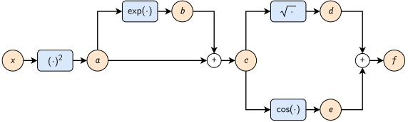
Computation graph of \(f(x) = \sqrt{x^2 + \exp(x^2)} + \cos(x^2 + \exp(x^2))\), with the intermediate variables \(a = x^2\), \(b = \exp(a)\), \(c = a + b\), \(d = \sqrt{c}\) and \(e = \cos(c)\), and \(f = d + e\). Adapted from: Mathematics for Machine Learning, Example 5.14
This is the same kind of thinking process that occurs when applying the chain rule. Note that the preceding set of equations requires fewer operations than a direct implementation of the function \(f(x)\).
The backward pass then computes the derivative of the output with respect to each variable, from \(f\) back to \(x\). Each step needs only the derivatives of the elementary operations with respect to their inputs:
\[\frac{\partial a}{\partial x} = 2x, \quad \frac{\partial b}{\partial a} = \exp(a), \quad \frac{\partial c}{\partial a} = 1 = \frac{\partial c}{\partial b}, \quad \frac{\partial d}{\partial c} = \frac{1}{2\sqrt{c}}, \quad \frac{\partial e}{\partial c} = -\sin(c), \quad \frac{\partial f}{\partial d} = 1 = \frac{\partial f}{\partial e}\]Following the arrows of the graph backwards, the chain rule sums the contributions of all the paths that leave a variable:
\[\begin{align*} \frac{\partial f}{\partial c} & = \frac{\partial f}{\partial d} \frac{\partial d}{\partial c} + \frac{\partial f}{\partial e} \frac{\partial e}{\partial c} \, , \\ \frac{\partial f}{\partial b} & = \frac{\partial f}{\partial c} \frac{\partial c}{\partial b} \, , \\ \frac{\partial f}{\partial a} & = \frac{\partial f}{\partial b} \frac{\partial b}{\partial a} + \frac{\partial f}{\partial c} \frac{\partial c}{\partial a} \, , \\ \frac{\partial f}{\partial x} & = \frac{\partial f}{\partial a} \frac{\partial a}{\partial x} \, . \end{align*}\]As an example, at \(x = 1\) the forward pass computes \(a = 1\), \(b = \exp(1) = 2.718\), \(c = 3.718\), \(d = 1.928\), \(e = -0.838\) and \(f = 1.090\). The backward pass then gives \(\partial f / \partial c = 1/(2d) - \sin(c) = 0.805\), \(\partial f / \partial b = \partial f / \partial c = 0.805\), \(\partial f / \partial a = b \, \partial f / \partial b + \partial f / \partial c = 2.992\) and \(\partial f / \partial x = 2x \, \partial f / \partial a = 5.98\), the value of the closed-form derivative above at \(x = 1\). Each step of the backward pass costs a few operations, so the derivative costs about as much as the function itself.
This backward pass is the reverse mode of automatic differentiation. One pass from the output back to the inputs gives the derivatives of the output with respect to all the inputs, at a small constant factor of the cost of the function. The forward mode propagates the derivatives from one input to all the outputs instead, so it needs one pass per input. A neural network has millions of parameters and one scalar loss, so it is trained with the reverse mode, of which backpropagation is the special case for neural networks.
In practice, autodiff libraries such as PyTorch’s autograd apply the chain rule to the derivatives of the elementary operations of the forward pass. Thus, contrary to the derivation of the errors above, the derivatives of the loss and activation functions do not have to be specified explicitly.
Instead, a computational graph (a DAG) is created dynamically, where nodes are added to the graph as the modules’ forward methods are called. The backward propagation is then computed by applying the chain rule to the derivatives (grad_fn) of the nodes in the computational graph. Recursive calls add new nodes to the graph for every call, and conditional calls may add different nodes at each forward pass; therefore, the computational graph cannot be extracted from the model definition directly (see an example here).
Finally, when tensor.backward() is called, it recursively computes the gradients up to the leaf nodes of the graph. When this process ends, the computational graph is discarded, and a new one may be created via a new forward call (unless retain_graph=True is set in the backward function). For more details, Chi-Feng Wang’s post gives an illustrative example of the automatic differentiation graph, and the Princeton course COS 324 on automatic differentiation a thorough explanation of the whole process.
Storing a computational graph is also useful for activation checkpointing, where one needs to recompute a module’s output during the backward pass, as it is discarded during the forward pass to save memory. A good example of activation checkpointing based on the reentrant and non-reentrant PyTorch implementations can be found in the post How Activation Checkpointing enables scaling up training deep learning models.
It also follows that inference requires less memory than training. The derivative of the weights of a layer, \(x^{(l-1)} (\delta^{(l)})^T\), needs the input of the layer (self.x of the linear layer above). Therefore, training saves the activations of all layers in the computational graph until the backward pass, while inference can discard them as soon as the next layer is computed.
The two layers above are enough for a minimal form of reverse-mode autodiff, whose elementary operations are the layers. A multi-layer perceptron (MLP) stores its layers in a list, in the order of the forward pass, which computes \(f^{(L+1)} \circ ... \circ f^{(1)}\). This list plays the role of the computational graph, and each layer saves what its backward pass needs (self.x and self.z), as the nodes of PyTorch’s graph do. The backward method then runs the layers in reverse order, from the error \(\delta^{(L+1)}\) of the output layer to the first layer:
class MLP:
    def __init__(self, sizes):
        self.layers = []
        for n_in, n_out in zip(sizes[:-1], sizes[1:]):
            self.layers += [Linear(n_in, n_out), ReLU()]
        self.layers.pop()  # no activation after the output layer

    def forward(self, x):
        for layer in self.layers:
            x = layer.forward(x)
        return x

    def backward(self, delta):
        for layer in reversed(self.layers):
            delta = layer.backward(delta)
        return delta  # the derivative of the loss with respect to the input

    def parameters(self):
        return [theta for layer in self.layers for theta in layer.parameters()]
Contrary to PyTorch, the graph is fixed by the model definition, and the derivatives of each layer are written by hand. As an example, MLP([2, 16, 16, 1]) builds a network with \(D = 2\) inputs, \(L = 2\) hidden layers of \(K = 16\) ReLU neurons and one output. The finite differences above can check its derivatives: on a small network, the derivatives computed both ways agree to about \(10^{-10}\).
For completeness, very good step-by-step overviews of the backpropagation theory applied to a real example can be found in Hooks for autograd saved tensors and PyTorch Autograd: Backpropagation.
Optimizers
Backpropagation computes the gradient \(g_t\) of the loss with respect to the parameters \(\theta\) of the network (all its weights and biases), at the step \(t\) of the training. An optimizer uses this gradient to update the parameters. The simplest one, gradient descent (GD), presented in the post Algebra for ML, takes a step against the gradient, of a size set by the learning rate \(\eta\):
\[\theta_t = \theta_{t-1} - \eta \, g_t\]In GD, \(g_t\) is the gradient of the loss over all \(N\) training samples, so each step follows the exact gradient, but costs a pass over the whole dataset. Stochastic gradient descent (SGD), presented in the post on linear regression, computes it on one sample or, in practice, on a mini-batch of \(B\) samples drawn at random (mini-batch SGD), which gives a noisy but unbiased estimate of the gradient, \(N/B\) times cheaper to compute. Momentum smooths the steps of SGD: it keeps a decaying sum \(m_t\) of the past gradients, and steps along it:
\[\begin{align*} m_t & = \mu \, m_{t-1} + g_t \\ \theta_t & = \theta_{t-1} - \eta \, m_t \end{align*}\]where the momentum \(\mu\) is usually 0.9 (0.95 to 0.99 with dropout). Gradients that agree from step to step add up, while those that change sign cancel out, which also speeds up training along the long, narrow valleys of the loss.
In code, an optimizer holds the parameters of a model. Its zero_grad method resets their derivatives, which the backward pass accumulates, and its step method updates them. The following SGD implements the equations above, and plain SGD for \(\mu = 0\), its default:
class Optimizer:
    def __init__(self, parameters, eta):
        self.parameters, self.eta = parameters, eta

    def zero_grad(self):
        for theta in self.parameters:
            theta.grad.fill(0)

class SGD(Optimizer):
    def __init__(self, parameters, eta, mu=0):
        super().__init__(parameters, eta)
        self.mu = mu
        self.m = [np.zeros_like(theta.data) for theta in parameters]

    def step(self):
        for theta, m in zip(self.parameters, self.m):
            m[:] = self.mu * m + theta.grad
            theta.data -= self.eta * m
Adam (adaptive moment estimation), introduced in Adam: A Method for Stochastic Optimization, keeps the momentum \(m_t\) as a running average of the gradients instead of a sum, and a running average \(v_t\) of their squares. It thus combines momentum, for the first moment, with RMSProp, which divides the learning rate of each weight by a running average of the magnitudes of its recent gradients, for the second moment. It divides the step of each parameter by \(\sqrt{v_t}\), so that each parameter moves by at most about \(\eta\) per step, whatever the scale of its gradients, as \(\vert \mathbb{E}[g_t] \vert \le \sqrt{\mathbb{E}[g_t^2]}\) (section 2.1 of the paper). Its update is given by (Algorithm 1 in the paper, which writes \(\alpha\) for \(\eta\)):
\[\begin{align*} m_t & = \beta_1 m_{t-1} + (1 - \beta_1) \, g_t \\ v_t & = \beta_2 v_{t-1} + (1 - \beta_2) \, g_t^2 \\ \hat{m}_t & = m_t / (1 - \beta_1^t) \\ \hat{v}_t & = v_t / (1 - \beta_2^t) \\ \theta_t & = \theta_{t-1} - \eta \, \hat{m}_t / (\sqrt{\hat{v}_t} + \epsilon) \end{align*}\]where the square, the root and the division apply to each entry. Note that \(v_t\) estimates the second moment of the gradient, its uncentered variance, and not the second derivative (the curvature), which would be too expensive to compute. As \(m_0 = v_0 = 0\), both averages are biased toward zero in the first steps, and \(\hat{m}_t\) and \(\hat{v}_t\) correct this bias. The paper suggests \(\eta = 0.001\), \(\beta_1 = 0.9\), \(\beta_2 = 0.999\) and \(\epsilon = 10^{-8}\), the default values of the code:
class Adam(Optimizer):
    def __init__(self, parameters, eta=1e-3, beta1=0.9, beta2=0.999, eps=1e-8):
        super().__init__(parameters, eta)
        self.beta1, self.beta2, self.eps, self.t = beta1, beta2, eps, 0
        self.m = [np.zeros_like(theta.data) for theta in parameters]
        self.v = [np.zeros_like(theta.data) for theta in parameters]

    def step(self):
        self.t += 1
        for theta, m, v in zip(self.parameters, self.m, self.v):
            m[:] = self.beta1 * m + (1 - self.beta1) * theta.grad
            v[:] = self.beta2 * v + (1 - self.beta2) * theta.grad**2
            m_hat = m / (1 - self.beta1**self.t)
            v_hat = v / (1 - self.beta2**self.t)
            theta.data -= self.eta * m_hat / (np.sqrt(v_hat) + self.eps)
The following picture compares the paths of GD, momentum and Adam on a loss with a long, narrow valley:
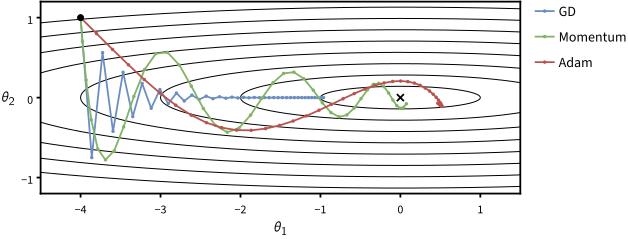
The first 40 steps of GD (\(\eta = 0.035\)), momentum (\(\eta = 0.006\), \(\mu = 0.9\)) and Adam (\(\eta = 0.2\), with the default \(\beta_1\), \(\beta_2\) and \(\epsilon\)) on the loss \(\theta_1^2/2 + 25 \theta_2^2\) (black contours), with its exact gradient, from the same starting point (black dot) toward the minimum (cross). GD zig-zags across the narrow valley and moves slowly along it, momentum oscillates across the valley but gains speed along it, and Adam moves each parameter by about \(\eta\) per step at first, whatever the scale of its gradient.
In practice, Adam needs less tuning of the learning rate than SGD, and Adam or its variants train most Transformers, while SGD with momentum remains common for CNNs. However, in some cases, Adam does not converge to the optimal solution, but SGD does (Reddi et al., 2018), and switching from Adam to SGD during training can generalize better than Adam alone (Keskar and Socher, 2017).
Adam keeps two running averages per parameter, while momentum keeps one and plain SGD none: for a model of a billion parameters, the averages of Adam take 8 GB in FP32. Its variant AdamW, from Decoupled Weight Decay Regularization, shrinks the weights at every step (weight decay) directly, instead of adding an L2 regularization term to the gradient, which Adam would rescale.
Training Loop
The training loop needs one more piece, the loss. The squared loss of the backpropagation section, averaged over the \(B\) samples of a mini-batch, is the MSE:
\[\mathcal{L} = \frac{1}{B} \sum_{n=1}^{B} (y_n - \hat{y}_n)^2\]where \(\hat{y}_n\) is the output of the network for the sample \(n\). The backward method of the loss returns the error of the output layer, \(\delta_n^{(L+1)} = -2 (y_n - \hat{y}_n)\) as in the backpropagation section, divided by \(B\) as the loss is a mean:
class MSELoss:
    def forward(self, y_hat, y):
        self.y_hat, self.y = y_hat, y  # saved for the backward pass
        return np.mean((y - y_hat)**2)

    def backward(self):
        B = self.y.size  # samples in the mini-batch, with one output each
        return -2 * (self.y - self.y_hat) / B
For classification, a softmax output with the cross-entropy loss gives an error of the same form, \(\hat{y}_n - y_n\), where \(\hat{y}_n\) holds the predicted probabilities of the classes and \(y_n\) is the one-hot vector of the true class.
Then, the loop. The following example trains an MLP on a continuous version of XOR: points drawn uniformly in \([-1, 1]^2\), with the target 1 when their two coordinates have different signs and 0 otherwise. As for XOR, no line separates the two classes. At each step, the loop draws a random mini-batch of \(B = 32\) samples, resets the derivatives, and runs the forward pass, the loss, the backward pass and the optimizer step, in the order of a PyTorch training loop:
def xor_data(N):
    x = np.random.uniform(-1, 1, (N, 2))
    y = (x[:, 0] * x[:, 1] < 0).astype(float).reshape(N, 1)  # 1 if the signs differ
    return x, y

np.random.seed(0)
N, B = 1024, 32  # training samples, mini-batch size
x, y = xor_data(N)
x_test, y_test = xor_data(256)
model = MLP([2, 16, 16, 1])
loss_fn = MSELoss()
optimizer = Adam(model.parameters(), eta=0.01)

for step in range(2000):
    n = np.random.choice(N, B, replace=False)  # samples of a random mini-batch
    optimizer.zero_grad()
    loss = loss_fn.forward(model.forward(x[n]), y[n])
    model.backward(loss_fn.backward())
    optimizer.step()
    if step % 500 == 0:
        print(f"step {step}: loss {loss:.4f}")

print("test accuracy:", np.mean((model.forward(x_test) > 0.5) == y_test))
With \(B = N\), the same loop runs GD. After 2,000 steps, the network classifies 99.2% of the 256 test points correctly, with an output above 0.5 for the target 1, and the two misclassified points lie within 0.006 of an axis, where the class changes. SGD with momentum, SGD(model.parameters(), eta=0.1, mu=0.9), classifies 98.8% of them correctly.
To find more about the topic, the Deep Learning book by Goodfellow, Bengio and Courville covers feedforward networks and backpropagation (chapter 6) and optimization (chapter 8), and the Mathematics for Machine Learning book covers backpropagation and automatic differentiation (section 5.6).