Dropout, CNNs, Skip Connections and Embeddings
In 2012, the network AlexNet, presented in the paper ImageNet Classification with Deep Convolutional Neural Networks, won the ImageNet competition (ILSVRC-2012) with a top-5 test error of 15.3%, against 26.2% for the second-best entry. It was a convolutional neural network of 60 million parameters, trained on two GPUs, with dropout to reduce overfitting in its fully connected layers. Three years later, ResNet added skip connections, which made networks of more than 100 layers trainable.
The post Deep Neural Networks, Backpropagation and Optimization presented fully connected networks and how they are trained. This post covers dropout, convolutional neural networks (CNNs), skip connections and embeddings, and then the loss functions of tasks other than regression and classification, such as learning embeddings and segmenting images.
Dropout
A network with many parameters is prone to overfitting: it learns the noise of the training data, and generalizes poorly to new data. Dropout, described in the paper Dropout: A Simple Way to Prevent Neural Networks from Overfitting, is a method that drops neurons (in different layers) with a given probability \(p\) at training time. For each training sample in a mini-batch, a new thinned network is sampled, made of the neurons that are kept.
The outputs of the kept neurons are scaled by \(1/(1-p)\), so that their expected value is the same at training and inference time. An output \(x_j^{(l)}\) is kept with probability \(1-p\), so its expected value is \((1-p) \times x_j^{(l)}/(1-p) = x_j^{(l)}\). At inference time, all neurons are used, and no dropout is applied. This scaling at training time is known as inverted dropout; note that the paper scales the weights at inference time instead, and writes \(p\) for the probability of keeping a unit.
A simple code snippet to explain this follows the NumPy layers of the post on deep neural networks, with a forward and a backward method, and the code of this post reuses their classes Parameter, Linear, ReLU and MLP. First, the base class Layer gives the layers without parameters an empty list of parameters. Then, the forward method of Dropout draws a mask that keeps each unit with probability \(1-p\), scaled by \(1/(1-p)\), and multiplies the input by it. As the output is the input times this mask, the backward method multiplies the derivative of the loss by the same mask, so that the dropped units get no gradient:
class Layer:  # a layer without parameters
    def parameters(self):
        return []

class Dropout(Layer):
    def __init__(self, p=0.5):
        self.p, self.training = p, True  # training is False at inference time

    def forward(self, x):
        if not self.training:
            return x
        self.mask = (np.random.rand(*x.shape) >= self.p) / (1 - self.p)  # scaled kept units
        return x * self.mask

    def backward(self, dx):
        return dx * self.mask
The flag training plays the role of the train() and eval() methods of a PyTorch module.
Dropout helps reduce overfitting, as the network learns to never rely on any given activation, so it learns redundant ways of solving the task with multiple neurons. As a side effect, it leads to sparse activations, similar to an L1 regularization of the activations (section 7.2 of the paper). For linear regression, it is equivalent in expectation to an L2 regularization of the weights, i.e. ridge regression (section 9.1).
In practice, dropout works best with max-norm regularization (an upper bound on the norm of the incoming weights of each neuron), a large decaying learning rate and a high momentum (0.95 to 0.99 instead of the usual 0.9). Dropping 20% of the input units and 50% of the hidden units was often found to be close to optimal in the original publication. However, a dropout network takes 2 to 3 times longer to train than a standard network of the same architecture, because it requires many more epochs, as parameter updates are very noisy.
Because the fully connected layers hold most of the parameters of a network such as the CNNs below, they are the most prone to overfitting, and dropout is often applied to them. The following picture illustrates a standard network (left) and one of the thinned networks that dropout samples from it (right):
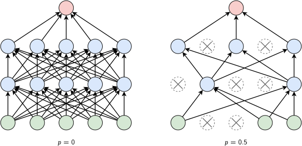
Dropout. Left: a standard network with two hidden layers (\(p = 0\)). Right: a thinned network produced by dropout with \(p = 0.5\), where \(p\) is the probability of dropping a unit: the crossed units are dropped, with their connections. Adapted from: Dropout: A Simple Way to Prevent Neural Networks from Overfitting
The network on the left has 15 units that dropout can drop, its 5 inputs and 10 hidden units. Each training sample thus uses one of \(2^{15} = 32{,}768\) thinned networks, which all share the same weights. At inference time, the full network with the scaled outputs approximates the average of the predictions of all these thinned networks, which is computationally much less expensive than the regular model averaging of multiple trained DNNs.
Convolutional Neural Networks
The disadvantage of large neural networks is that they have a very high number of parameters, so they may require lots of data to be trained. In some scenarios, local connectivity should suffice. For example, in an audio stream, it is natural to process an input stream \(x^{(0)}[n]\) by running it through a linear time-invariant filter, whose output \(x^{(1)}[n]\) is given by the convolution of the input \(x^{(0)}[n]\) and the filter \(h[n]\), as:
\[x^{(1)}[n] = \sum_u h[u]x^{(0)} [n-u]\]The filter \(h\) is local, i.e. \(h[u]=0\) for \(\vert u \vert \ge r\). By choosing an appropriate type of filter, one can bring out various aspects of the underlying signal, e.g. smooth features by averaging, or enhance differences between neighboring elements by using a high-pass filter. As an example, the filter \(h[-1] = h[0] = h[1] = 1/3\) averages three neighbors, and the filter \(h[0] = 1\), \(h[1] = -1\) computes the difference \(x^{(0)}[n] - x^{(0)}[n-1]\). An analogous scenario applies to a picture:
\[x^{(1)}[n,m] = \sum_{u,v} h[u,v]x^{(0)} [n-u,m-v]\]The output \(x^{(1)}\) at position \([n, m]\) only depends on the values of the input \(x^{(0)}\) at positions close to \([n, m]\). So a fully connected network is no longer needed, but only one that represents the local structure, leading to fewer parameters to deal with.
This structure implies that the same filter (i.e., not only the same connection pattern but also the same weights) should be used at every position! This is called weight sharing, and it reduces the number of parameters even further, as a pattern such as an edge is detected by the same filter wherever it appears in the input. The following picture shows the difference between a locally (sparsely) connected and a fully connected layer:
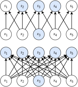
Sparse and full connectivity, viewed from below. Top: a locally connected layer with a kernel of width 3, where the input \(x_3\) affects only the outputs \(s_2\), \(s_3\) and \(s_4\). Bottom: a fully connected layer, where \(x_3\) affects every output. Adapted from: Deep Learning, I. Goodfellow, Y. Bengio and A. Courville, Figure 9.2
In the picture, the inputs \(x_i\) and the outputs \(s_i\) stand for the \(x^{(0)}\) and \(x^{(1)}\) of the text. The fully connected layer has \(5 \times 5 = 25\) weights, one per connection. The locally connected layer has 13 connections, as each output reads at most 3 inputs, and, with weight sharing, only the 3 weights of its filter.
It is common to not only compute the output of a single filter but to use multiple filters. The various outputs are called channels (or feature maps). This introduces some additional parameters into the model, as each filter has its own weights, and spans all the channels of its input.
With several channels, the result is not a 2D output in the next level, but in fact a 3D output. Layer after layer, there are increasingly more channels but a smaller “footprint”. In brief, applying local connectivity to a 2D input dataset on a deep neural network leads to the following final structure, a convolutional neural network (CNN):
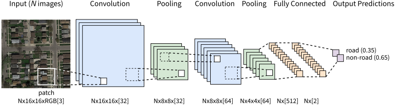
A CNN that classifies \(16 \times 16\) RGB patches of a satellite image as road or non-road: two stages of convolution and pooling, two fully connected layers, and the output probabilities of the two classes. Each label gives the shape of the data after a layer for \(N\) input images, with the number of channels or units in brackets.
Notice the three types of operations involved:
- convolutional layer: applies a convolution operation to the input, passing the result to the next layer. The convolution emulates the response of an individual neuron to visual stimuli;
- convolution is a mathematical operation on two functions that produces a third function, which expresses how the shape of one is modified by the other. In practice, the convolutional layers of deep learning libraries compute a cross-correlation, \(x^{(1)}[n,m] = \sum_{u,v} h[u,v] \, x^{(0)}[n+u,m+v]\), i.e. a convolution with a flipped filter (Deep Learning book, section 9.1); as the filter is learned, the two are equivalent;
- pooling: combines the outputs of neuron clusters at one layer into a single neuron in the next layer;
- a very common operation is max pooling, which uses the maximum value of each cluster of neurons at the prior layer, e.g. of each \(2 \times 2\) window in the picture;
- fully connected: similar to a multi-layer perceptron, providing the universal approximator function.
The size of each feature map typically gets smaller and smaller as the data proceeds through the layers, either due to the handling of the boundary or because the network may perform subsampling. Along each dimension, the size of the output of a convolution or a pooling is given by:
\[d_{\text{out}} = \left\lfloor \frac{d_{\text{in}} + 2 \times \text{padding} - \text{kernel size}}{\text{stride}} \right\rfloor + 1\]where \(d_{\text{in}}\) is the size of the input and the kernel size is the size of the filter or of the pooling window. The stride is the step by which the window moves, and the padding is the number of zeros added on each side of the input. In the picture, the convolutions pad their input so that the output keeps the size of \(16 \times 16\), and each max pooling of \(2 \times 2\) with a stride of 2 halves it, to \(\lfloor (16 - 2)/2 \rfloor + 1 = 8\) and then 4.
Weight sharing makes a convolutional layer much smaller than a fully connected one. Consider the first layer of the network above, which turns a \(16 \times 16\) RGB patch (768 inputs) into 32 channels of \(16 \times 16\) (8,192 outputs). A fully connected layer between them has \(768 \times 8{,}192\) weights and 8,192 biases, about 6.3 million parameters. A convolutional layer with 32 filters of \(3 \times 3\) pixels over the 3 color channels has \(32 \times (3 \times 3 \times 3 + 1) = 896\), 7,000 times fewer, and the same 896 for an input of any size. The fully connected layers, instead, hold most of the parameters of a CNN. The first one connects the \(4 \times 4 \times 64 = 1{,}024\) outputs of the last pooling layer to 512 units, with \(1{,}024 \times 512 + 512 = 524{,}800\) parameters, more than all the convolutional layers together.
Training is done with backpropagation, ignoring that some weights are shared and considering each weight on each edge to be an independent variable. Once the gradient has been computed for this network with independent weights, the gradients of all edges that share the same weight are summed up. This gives the gradient for the network with weight sharing, as the loss depends on the shared weight through each of these edges.
For one channel, with the cross-correlation \(x^{(1)}[n,m] = \sum_{u,v} h[u,v] \, x^{(0)}[n+u,m+v]\) of deep learning libraries and the error \(\delta[n,m] = \partial \mathcal{L} / \partial x^{(1)}[n,m]\) of the output, the chain rule gives the derivatives of the loss with respect to the filter and to the input as:
\[\frac{\partial \mathcal{L}}{\partial h[u,v]} = \sum_{n,m} \delta[n,m] \, x^{(0)}[n+u,m+v], \hspace{1cm} \frac{\partial \mathcal{L}}{\partial x^{(0)}[n,m]} = \sum_{u,v} \delta[n-u,m-v] \, h[u,v]\]The first sum adds up the derivatives of the shared weight \(h[u,v]\) over all the positions of the filter, as described above. The second is a convolution of the error with the filter, and not a cross-correlation, over all the positions where they overlap (a full convolution). Thus, the backward pass of a convolutional layer is also a convolution, from the output channels to the input channels.
Both passes are computed as matrix products. The windows of the input that the filter covers, after the padding, are gathered into a matrix with one window per row (a method known as im2col), and the convolution becomes the product of this matrix with the matrix of the filters, computed by the same optimized routines as the matrix products of a fully connected layer. In NumPy, sliding_window_view gives these windows as a view of the input, without copying it, and tensordot copies them into such a matrix and multiplies it by the filters, over the two dimensions of the window and the input channels. The images have the shape \(B \times H \times W \times C\) (\(N \times 16 \times 16 \times 3\) in the picture above), with the channels last, and the layer has a stride of 1, as the convolutions of the picture:
from numpy.lib.stride_tricks import sliding_window_view

class Conv2d:
    def __init__(self, c_in, c_out, k, padding=0):
        std = np.sqrt(2 / (k * k * c_in))  # He initialization, for ReLU
        self.W = Parameter(np.random.normal(0, std, (k, k, c_in, c_out)))
        self.b = Parameter(np.zeros(c_out))
        self.k, self.padding = k, padding

    def forward(self, x):  # x: B x H x W x C_in, with a stride of 1
        p = self.padding
        x = np.pad(x, ((0, 0), (p, p), (p, p), (0, 0)))
        # windows of shape B x H_out x W_out x C_in x k x k
        self.windows = sliding_window_view(x, (self.k, self.k), axis=(1, 2))
        z = np.tensordot(self.windows, self.W.data, axes=([4, 5, 3], [0, 1, 2]))
        return z + self.b.data

    def backward(self, delta):  # delta: B x H_out x W_out x C_out
        k, p = self.k, self.padding
        # sum over the images and the positions, of shape C_in x k x k x C_out
        dW = np.tensordot(self.windows, delta, axes=([0, 1, 2], [0, 1, 2]))
        self.W.grad += dW.transpose(1, 2, 0, 3)
        self.b.grad += delta.sum(axis=(0, 1, 2))
        delta = np.pad(delta, ((0, 0), (k - 1, k - 1), (k - 1, k - 1), (0, 0)))
        windows = sliding_window_view(delta, (k, k), axis=(1, 2))
        # full convolution, with the flipped filters
        dx = np.tensordot(windows, self.W.data[::-1, ::-1], axes=([4, 5, 3], [0, 1, 3]))
        return dx[:, p:dx.shape[1] - p, p:dx.shape[2] - p]  # without the padding

    def parameters(self):
        return [self.W, self.b]
The backward method pads the error with k - 1 zeros on each side, for a kernel size k, and multiplies its windows by the flipped filters, which computes the full convolution above, and then removes the padding of the input. Then comes the max pooling layer, which has no parameters. Its forward method keeps the maximum of each window of \(2 \times 2\), and its backward method passes the derivative of each output to the position of that maximum only, as the other inputs of the window do not change the output:
class MaxPool2d(Layer):  # windows of 2 x 2 with a stride of 2
    def forward(self, x):
        self.shape = x.shape  # saved for the backward pass
        B, H, W, C = x.shape
        x = x.reshape(B, H // 2, 2, W // 2, 2, C).transpose(0, 1, 3, 5, 2, 4)
        x = x.reshape(B, H // 2, W // 2, C, 4)  # each window in the last axis
        self.idx = x.argmax(axis=-1)  # the position of the maximum of each window
        return x.max(axis=-1)

    def backward(self, delta):
        B, H, W, C = self.shape
        dx = np.zeros((B, H // 2, W // 2, C, 4))
        np.put_along_axis(dx, self.idx[..., None], delta[..., None], axis=-1)
        dx = dx.reshape(B, H // 2, W // 2, C, 2, 2).transpose(0, 1, 4, 2, 5, 3)
        return dx.reshape(B, H, W, C)
Finally, Flatten turns the feature maps of each image into one vector, the input of the fully connected layers, and Sequential builds a network from a list of layers, with the forward, backward and parameters methods of the MLP of the DNN post. And that is all: the CNN of the picture above, with ReLU activations, is given by:
class Flatten(Layer):
    def forward(self, x):
        self.shape = x.shape  # saved for the backward pass
        return x.reshape(len(x), -1)

    def backward(self, delta):
        return delta.reshape(self.shape)

class Sequential(MLP):
    def __init__(self, *layers):
        self.layers = list(layers)

model = Sequential(Conv2d(3, 32, 3, padding=1), ReLU(), MaxPool2d(),
                   Conv2d(32, 64, 3, padding=1), ReLU(), MaxPool2d(), Flatten(),
                   Linear(4 * 4 * 64, 512), ReLU(), Linear(512, 2))
The model has 545,218 parameters, of which the first fully connected layer holds the 524,800 counted above. On a small CNN made of these layers, the derivatives agree with finite differences to about \(10^{-9}\). In practice, deep learning libraries run these computations with optimized GPU kernels, and choose among several algorithms, such as im2col, the fast Fourier transform and Winograd’s minimal filtering (Lavin and Gray, 2015), depending on the sizes of the filters and of the images.
Skip Connections
An issue with very deep networks is that the performance of the model drops as the depth of the architecture increases. This is known as the degradation problem. It is not caused by overfitting, since the training error increases as well.
Possible reasons are vanishing and/or exploding gradients. One way to improve this is to use normalization techniques to ensure that gradients have healthy norms. However, the authors of ResNet observed the degradation problem even with normalization layers and healthy gradient norms. On the CIFAR-10 dataset, a plain network of 56 layers has a higher training error than one of 20 layers.
A better way to improve this is to provide layers of the network with the outputs of layers that are not directly connected to them. These connections skip some of the layers in the neural network and feed the output of one layer as the input of later layers, hence the name skip connections. In practice, the input to a given layer is the combination (typically via addition or concatenation) of the outputs of several previous layers.
With an addition, as in ResNet, a block of layers with the input \(x\) computes \(y = x + F(x)\), where \(F\) is the function of the skipped layers. These layers only need to learn a correction (a residual) to their input, which is easier to optimize than the whole mapping.
The addition also helps the backward pass. The derivative of the output of the block with respect to its input (its Jacobian matrix) is \(I + \partial F / \partial x\), where \(I\) is the identity matrix. Thus, the gradient of the loss with respect to the input of the block is given by:
\[\frac{\partial \mathcal{L}}{\partial x} = \frac{\partial \mathcal{L}}{\partial y} + \left( \frac{\partial F}{\partial x} \right)^T \frac{\partial \mathcal{L}}{\partial y}\]where the first term passes the gradient of the layers above to the layers below unchanged, even when the derivatives of the skipped layers are small. Over a stack of blocks, the paper Identity Mappings in Deep Residual Networks showed that the gradient at any block contains the gradient at the last block as an additive term (Eq. 5 in the paper). Therefore, it does not vanish, even when the weights are arbitrarily small.
In code, a residual block is a Sequential model of the skipped layers \(F\), whose output is added to its input. Its backward method follows the equation above: it adds the derivative of the loss with respect to the output of the block, \(\partial \mathcal{L} / \partial y\), to the derivative that the skipped layers return:
class Residual(Sequential):  # y = x + F(x), with the layers of F
    def forward(self, x):
        return x + super().forward(x)

    def backward(self, dy):
        return dy + super().backward(dy)
As an example, Residual(Conv2d(64, 64, 3, padding=1), ReLU(), Conv2d(64, 64, 3, padding=1)) followed by ReLU() is the basic block of ResNet, without its batch normalization layers. The padding keeps the size of the feature maps, so that \(x\) and \(F(x)\) can be added.
With a concatenation, as in DenseNet, each layer receives the feature maps of all the layers before it, so the number of channels grows with every layer. If each layer produces \(k\) feature maps (the growth rate), the layer \(H_l\) receives \(k_0 + k(l-1)\) of them, where \(k_0\) is the number of channels of the input of the block (DenseNet paper, section 3). The following picture illustrates a dense block of DenseNet:
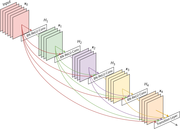
A 5-layer dense block of DenseNet with a growth rate of \(k = 4\): each layer \(H_i\) (BN-ReLU-Conv) takes the feature maps \(x_0, \ldots, x_{i-1}\) of all preceding layers as input and produces \(k\) new feature maps \(x_i\). The transition layer takes all of them. Adapted from: Densely Connected Convolutional Networks
In the picture, the input \(x_0\) has \(k_0 = 6\) feature maps and \(k = 4\), so the layer \(H_4\) receives \(6 + 4 \times 3 = 18\) feature maps, and the transition layer, which takes all of them, \(6 + 4 \times 4 = 22\). To sum up, an addition (ResNet) keeps the number of channels constant, while a concatenation (DenseNet) lets every layer read the feature maps of all the layers before it. The price of DenseNet is an input that grows with the depth of the block, which is why it uses small growth rates (\(k\) from 12 to 40 in its experiments).
Similarly, each layer of a dense block concatenates its input and the output of its function \(H_l\), along the channels. Its backward method splits the derivative of the loss along the same channels: the part of the input channels passes to the input unchanged, as with the addition of ResNet, and the rest goes through \(H_l\):
class Concat(Sequential):  # y = [x, H(x)] along the channels, with the layers of H
    def forward(self, x):
        self.c = x.shape[-1]  # channels of the input
        return np.concatenate([x, super().forward(x)], axis=-1)

    def backward(self, dy):
        return dy[..., :self.c] + super().backward(dy[..., self.c:])

block = Sequential(*[Concat(ReLU(), Conv2d(6 + 4 * l, 4, 3, padding=1)) for l in range(4)])
The dense block of the picture, with \(k_0 = 6\) and \(k = 4\), is the model block of four such layers, which take 6, 10, 14 and 18 channels and return the 22 channels that the transition layer takes. Each \(H_l\) is a ReLU followed by a \(3 \times 3\) convolution, without the batch normalization of DenseNet.
There is currently a plethora of different implementations of CNNs with several layouts of skip connections. To know more, the curious reader can have a look at ResNet, DenseNet and U-net.
Embeddings
Embeddings in machine learning are dense, low-dimensional vector representations of data (e.g., words, images, or users) that capture their semantic or contextual meaning in a continuous vector space. Similar data have close embeddings, and the difference between two embeddings can carry a meaning: in the paper that introduced Word2vec, Efficient Estimation of Word Representations in Vector Space, \(\text{vector}(\text{King}) - \text{vector}(\text{Man}) + \text{vector}(\text{Woman})\) is closest to \(\text{vector}(\text{Queen})\). Embeddings can be collected by passing input data (e.g., text, images) through a trained machine learning model (e.g., a neural network) and extracting the values from a specific intermediate layer, typically before the final output layer.
The most common data types and their embeddings are:
- words: Word2vec learns an embedding for each word of a vocabulary, from inputs that are one-hot vectors of the words, with one of two models:
- skipgram, which predicts the surrounding words from the current word: slower to train (“3 days” in the original paper), better at capturing semantic relationships, e.g. for ‘cat’ it returns ‘dog’ as a word with close embeddings;
- continuous bag of words (CBOW), which predicts the current word from the surrounding words: faster to train (“1 day” on the same data), better at capturing syntactic relationships between words, e.g. for ‘cat’ it returns ‘cats’;
- text (word sequences): BERT;
- non-textual sequences: Encoder-Decoders, e.g. LSTMs, RNNs;
- point cluster or array: Principal Component Analysis;
- images:
- in a classification task: the activation of the last layer before the layer that does logit/softmax, i.e. the input to the final layer, e.g. the 512 values of the first fully connected layer of the CNN above;
- in an image-to-image task, e.g. segmentation using a U-net: the activation of the last downsampling layer, which is the input of the first upsampling layer, i.e. the bottleneck of the network;
- audio: the frames of a spectrogram, or the tokens of a neural audio codec, detailed below;
- videos: a sequence of video frames stacked on a time dimension, i.e. a 5D input, which a 3D convolution takes with the shape (batch size, channels, time, height, width). Embeddings are collected similarly to a regular CNN, with 3D instead of 2D convolutions;
- graphs: the states of the nodes after several steps of message passing, detailed below.
An audio waveform is a long 1D sequence of samples (typically 16-bit integers at 16 to 48 kHz), too long to model directly. It is thus first turned into a shorter sequence of frames, in one of two ways. The first is a log-Mel spectrogram, a 2D time-frequency image of the waveform, fed to a CNN or Transformer encoder whose activations are the embeddings. E.g. Whisper resamples audio to 16 kHz and computes 80 Mel channels on 25 ms windows with a 10 ms stride. A vocoder turns a spectrogram back into a waveform, as in the text-to-speech model TorToise.
The second is a neural audio codec: a convolutional encoder downsamples the waveform into embeddings, and a decoder with transposed convolutions reconstructs it. In between, residual vector quantization (RVQ) turns each embedding into discrete tokens: the embedding is replaced by its nearest entry in a codebook, the residual is quantized with a second codebook, and so on. E.g. EnCodec turns 24 kHz audio into 75 embeddings per second, a 320-fold reduction, and the number of codebooks sets the bitrate (8 codebooks of 1,024 entries give 6 kbps). DAC compresses 44.1 kHz audio into 8 kbps of tokens. These tokens can be modeled like text, e.g. VALL-E does text-to-speech by predicting EnCodec tokens with a language model.
For a graph, the embedding of a node is given by its state after several steps of the message passing algorithm, and the embedding of a graph by a readout (e.g. sum, mean or max) over all node embeddings. A message passing step is given by:
\[x_i^{(k)} = \gamma^{(k)} \left( x_i^{(k-1)}, \Box_{j \in \mathcal{N}(i)} \, \psi^{(k)} \left( x_i^{(k-1)}, x_j^{(k-1)}, e_{j,i} \right) \right)\]where:
- \(x_i^{(k)}\) is the embedding of node \(i\) at message passing step \(k\);
- \(\mathcal{N}(i)\) is the set of neighbors of node \(i\);
- \(e_{j,i}\) is the embedding of the edge from node \(j\) to node \(i\);
- \(\Box\) is a differentiable, permutation-invariant function, e.g. sum, mean or max;
- and \(\gamma\) and \(\psi\) are differentiable functions such as DNNs or RNNs (LSTMs, GRUs).
Task-Specific Loss Functions
The choice of the loss function depends on the task. Regression tasks use the MSE of the post on linear regression, and classification tasks the cross-entropy of the post on deep neural networks. Other tasks need other losses: the contrastive and triplet losses to learn embeddings, the CTC loss for unsegmented sequences, and the focal and Dice losses for imbalanced classes and image segmentation. The following sections present them in this order, and a table at the end of the post compares them with the MSE, the MAE and the cross-entropy.
Contrastive Loss
The contrastive loss trains siamese networks, two copies of one network with shared weights, against pairs of inputs labeled as similar or dissimilar (1 or 0). It is formulated in terms of the similarity label \(y\) (1 for similar, 0 for dissimilar) and the Euclidean distance \(\delta\) between the embeddings of the two inputs, as:
\[L = \frac{1}{2} ⋅y⋅\delta^2 + \frac{1}{2} ⋅(1−y)⋅\max(0,m-\delta)^2\]where \(m\) is a hyper-parameter (the margin). In practice, the loss pulls similar pairs together, towards a distance of 0, and pushes dissimilar pairs apart, and a dissimilar pair contributes to the loss only while its distance is below \(m\). The original paper is Dimensionality Reduction by Learning an Invariant Mapping, summarized in the publications bookmark.
The losses of this post follow the MSELoss of the post on deep neural networks: forward returns the loss averaged over a mini-batch of \(B\) samples, and backward returns its derivatives with respect to the inputs of the loss, from which the backward pass of the network starts. For the contrastive loss, the derivative with respect to the embedding \(e_1\) of the first input is \((y \, \delta - (1-y) \max(0, m - \delta)) (e_1 - e_2) / \delta\), and the one with respect to the embedding \(e_2\) of the second input is its opposite:
class ContrastiveLoss:
    def __init__(self, m=1.0):
        self.m = m  # margin

    def forward(self, e1, e2, y):  # embeddings of the B pairs, and their labels 1 or 0
        self.diff, self.y = e1 - e2, y
        self.d = np.linalg.norm(self.diff, axis=1)  # distances delta
        return np.mean(y * self.d**2 + (1 - y) * np.maximum(0, self.m - self.d)**2) / 2

    def backward(self):  # derivatives with respect to e1 and e2
        hinge = np.maximum(0, self.m - self.d)
        scale = self.y - (1 - self.y) * hinge / np.maximum(self.d, 1e-12)
        de1 = scale[:, None] * self.diff / len(self.d)
        return de1, -de1
Triplet Loss
Triplet loss is used in classification tasks where the number of classes is very large. Triplet loss helps by learning distributed embedding representations of data points such that, in the high-dimensional vector space, contextually similar data points are projected nearby, while dissimilar data points are projected far away from each other.
The network is trained against triplets of images: an anchor image of a person, a positive image, which is another image of the same person, and a negative image, which is a picture of another person. The Triplet Loss minimizes the Euclidean distance between the anchor and the positive, and maximizes the distance between the anchor and the negative. Tasks that can be performed: face recognition (“who is this person?”), verification (“are these the same person?”) and clustering (“find the most similar people”). The formulation is:
\[{\displaystyle {\mathcal {L}}\left(x,x^{+},x^{-}\right)=\operatorname {max} \left({\|\operatorname {f} \left(x\right)-\operatorname {f} \left(x^{+}\right)\|}^{2}-{\|\operatorname {f} \left(x\right)-\operatorname {f} \left(x^{-}\right)\|}^{2}+m ,0\right)}\]where \(x\) is an anchor input, \(x^{+}\) is a positive input of the same class as \(x\), \(x^{-}\) is a negative input of a different class from \(x\), \(m\) is a margin between positive and negative pairs, and \(f\) is an embedding. More details are given in the original paper, FaceNet: A Unified Embedding for Face Recognition and Clustering.
For a triplet with a positive loss, the derivatives with respect to \(f(x)\), \(f(x^+)\) and \(f(x^-)\) are \(2(f(x^-) - f(x^+))\), \(2(f(x^+) - f(x))\) and \(2(f(x) - f(x^-))\), and they are 0 for the other triplets. The default margin is the \(m = 0.2\) of the FaceNet paper:
class TripletLoss:
    def __init__(self, m=0.2):
        self.m = m  # margin

    def forward(self, a, p, n):  # embeddings of the B anchors, positives and negatives
        self.a, self.p, self.n = a, p, n
        loss = np.sum((a - p)**2, axis=1) - np.sum((a - n)**2, axis=1) + self.m
        self.active = (loss > 0)[:, None] / len(a)  # positive losses, divided by B
        return np.mean(np.maximum(loss, 0))

    def backward(self):  # derivatives with respect to a, p and n
        return (2 * (self.n - self.p) * self.active, 2 * (self.p - self.a) * self.active,
                2 * (self.a - self.n) * self.active)
The triplet loss is similar to, and often confused with, the contrastive loss, as both learn embeddings from examples of similar and dissimilar inputs. Yet, they constrain different distances. The contrastive loss constrains absolute distances: each similar pair is pulled towards a distance of 0, and each dissimilar pair is pushed beyond the margin \(m\). The triplet loss constrains relative distances: the squared distance of the anchor to the negative must exceed the one to the positive by the margin \(m\), whatever the distances themselves. In practice, the triplet loss considers the anchor-neighbor-distant triplets, while the contrastive loss deals with the anchor-neighbor and anchor-distant pairs of samples. As the FaceNet paper notes, a loss that pulls the faces of one person together “encourages all faces of one identity to be projected onto a single point in the embedding space”, while the triplet loss “allows the faces for one identity to live on a manifold”.
Connectionist Temporal Classification Loss
Connectionist Temporal Classification (CTC) is a classifier and loss function for noisy, unsegmented sequential input data, used to train recurrent neural networks (RNNs) such as LSTM networks to tackle sequence problems where the timing is variable. CTC was published by Graves et al. in 2006, in Connectionist Temporal Classification: Labelling Unsegmented Sequence Data with Recurrent Neural Networks.
At each time step, the network outputs the probability of each label and of an extra blank label (no label). The probability of a target sequence is the sum of the probabilities of all the alignments (one output per time step) that give the target once repeated labels and blanks are removed. As an example, with the blank written “−”, 7 of the 256 sequences of 4 outputs over the labels c, a, t and the blank give the target “cat”: “ccat”, “caat”, “catt”, “cat−”, “ca−t”, “c−at” and “−cat”. The blank also separates repeated labels: “l−l” gives “ll”, while “ll” gives “l”. The CTC loss is the negative logarithm of this probability, computed by dynamic programming, as the number of alignments grows quickly with the number of time steps (28 for 5 time steps).
The dynamic program runs over the target with a blank before, between and after its labels (“−c−a−t−” for “cat”), whose \(S = 2U + 1\) symbols, for a target of \(U\) labels, are the states of an alignment. An alignment starts in one of the first two states and ends in one of the last two, and at each time step it stays in its state, moves to the next one, or skips the blank between two different labels. The forward variable \(\alpha_t(s)\), the probability of the beginnings of the alignments that are in the state \(s\) at time \(t\), is thus given by (section 4.1 of the paper):
\[\alpha_t(s) = \left( \alpha_{t-1}(s) + \alpha_{t-1}(s-1) + [s \text{ may skip}] \, \alpha_{t-1}(s-2) \right) p^t_{l'_s}\]where \(l'_s\) is the label of the state \(s\), \(p^t_k\) is the probability of the label \(k\) at time \(t\) (\(y^t_k\) in the paper), and the last term counts only when \(l'_s\) is a label different from \(l'_{s-2}\). The probability of the target is the sum of \(\alpha_T(s)\) over the last two states. Similarly, the backward variable \(\beta_t(s)\) is the probability of the endings of these alignments after time \(t\), computed from \(t = T\) backwards (the paper’s \(\beta_t(s)\) also includes \(p^t_{l'_s}\)). Then, \(\alpha_t(s) \beta_t(s)\), normalized over \(s\), is the probability that an alignment is in the state \(s\) at time \(t\), and the derivative of the loss with respect to the logit of the label \(k\) at time \(t\) is \(p^t_k\) minus the sum of these probabilities over the states of the label \(k\) (Eq. 16 in the paper).
In code, each row of \(\alpha\) and \(\beta\) is scaled to a sum of 1, against underflow, and the scale factors of \(\alpha\) give the loss. First, log_softmax computes the logarithms of the probabilities without overflow. Then, CTCLoss computes the loss of one sequence and its derivatives with respect to the logits:
def log_softmax(z):  # along the last axis, shifted by the maximum against overflow
    z = z - z.max(axis=-1, keepdims=True)
    return z - np.log(np.sum(np.exp(z), axis=-1, keepdims=True))

class CTCLoss:  # one sequence, with the blank at index 0 of the C labels
    def forward(self, z, target):  # logits z: T x C; target: labels from 1 to C-1
        self.p = np.exp(log_softmax(z))
        l = np.zeros(2 * len(target) + 1, dtype=int)
        l[1::2] = target  # the target with a blank before, between and after its labels
        # an alignment may go from the state s-2 to s, over a blank
        skip = np.r_[False, False, (l[2:] != 0) & (l[2:] != l[:-2])]
        y = self.p[:, l]  # T x S: probability of the label of each state
        T, S = y.shape
        alpha, beta, scale = np.zeros((T, S)), np.zeros((T, S)), np.zeros(T)
        a = np.eye(S)[0]  # at t = -1, so that alignments start in the first two states
        beta[-1, -2:] = 1  # alignments end in the last two states
        for t in range(T):  # forward recursion, each row scaled to a sum of 1
            a = (a + np.r_[0, a[:-1]] + np.r_[0, 0, a[:-2]] * skip) * y[t]
            scale[t] = a.sum()
            alpha[t] = a = a / scale[t]
        for t in range(T - 1, 0, -1):  # backward recursion
            b = beta[t] * y[t]
            beta[t - 1] = b + np.r_[b[1:], 0] + np.r_[b[2:] * skip[2:], 0, 0]
            beta[t - 1] /= beta[t - 1].sum()
        self.gamma, self.labels = alpha * beta, np.eye(z.shape[1])[l]
        return -np.sum(np.log(scale)) - np.log(alpha[-1, -2:].sum())

    def backward(self):  # derivative with respect to the logits
        gamma = self.gamma / self.gamma.sum(axis=1, keepdims=True)  # state probabilities
        return self.p - gamma @ self.labels
On short sequences, the loss agrees with the sum over all the \(C^T\) alignments, and its derivatives with finite differences. A mini-batch averages the losses of its sequences.
Focal Loss
Focal Loss (Lin et al., 2017) is an extension of the Cross-Entropy Loss designed to address class imbalance, a common issue in e.g. dense object detection and medical image segmentation, where the background (non-lesion regions) is much more prevalent than the foreground (lesion regions). In dense detection, a detector evaluates about 100,000 candidate locations per image, and the paper gives an imbalance of 1:1000 between foreground and background as an example. Focal Loss focuses on hard-to-classify examples and down-weights the loss contribution from easy examples. For binary classification, it is defined as (Eq. 5 in the paper):
\[\mathcal{L}_{\text{focal}} = -\alpha_t (1 - p_t)^\gamma \log(p_t)\]where:
- \(p_t\) is the model’s estimated probability for the true class.
- \(\alpha_t\) is a balancing factor, equal to \(α\) for the positive class and to \(1-α\) for the negative class (especially useful for imbalanced datasets).
- \(γ\) is the focusing parameter, usually set to 2, which adjusts the focus on hard-to-classify examples.
In practice, the factor \((1 - p_t)^\gamma\) is close to 0 for well-classified examples, where \(p_t\) is close to 1, and close to 1 for misclassified examples. With \(\gamma = 2\), an example classified with \(p_t = 0.9\) has a loss 100 times lower than with the cross-entropy, as \((1 - 0.9)^2 = 0.01\), and one classified with \(p_t \approx 0.968\) a loss 1,000 times lower (section 3.2 of the paper). A misclassified example with \(p_t = 0.1\) keeps 81% of its loss. Thus, the many easy examples of the background no longer dominate the loss. With \(\gamma = 0\), the focal loss is the cross-entropy weighted by \(\alpha_t\) (Eq. 3 in the paper). For multi-class classification, the same formula applies, with one balancing factor per class, \(\alpha_t\) being the one of the true class. The following picture shows the focal loss for several values of \(\gamma\):
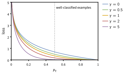
The focal loss as a function of \(p_t\), with \(\alpha_t = 1\), for values of \(\gamma\) from 0, the cross-entropy, to 5. A larger \(\gamma\) lowers the loss of the well-classified examples (\(p_t > 0.5\)) the most, which puts more focus on the misclassified ones. Inspired by: Focal Loss for Dense Object Detection
For softmax outputs, the chain rule through \(p_t\) gives the derivative of the focal loss with respect to the logits \(z\):
\[\frac{\partial \mathcal{L}_{\text{focal}}}{\partial z} = \alpha_t \left( \gamma (1 - p_t)^{\gamma - 1} p_t \log(p_t) - (1 - p_t)^\gamma \right) (y - p)\]where \(p\) is the vector of the predicted probabilities and \(y\) the one-hot vector of the true class. With \(\gamma = 0\) and \(\alpha_t = 1\), it is \(p - y\), the derivative of the cross-entropy. The argument alpha holds one balancing factor per class, e.g. np.array([0.75, 0.25]) for the \(\alpha = 0.25\) that the paper uses with \(\gamma = 2\), the class 1 being the positive one:
class FocalLoss:
    def __init__(self, gamma=2.0, alpha=None):
        self.gamma, self.alpha = gamma, alpha  # alpha: one factor per class, or None

    def forward(self, z, y):  # logits z and one-hot targets y, of shape B x C
        logp = log_softmax(z)
        self.p, self.y = np.exp(logp), y
        self.logpt = np.sum(logp * y, axis=1, keepdims=True)  # log(p_t)
        self.at = 1 if self.alpha is None else y @ self.alpha[:, None]  # alpha_t
        return -np.mean(self.at * (1 - np.exp(self.logpt))**self.gamma * self.logpt)

    def backward(self):  # derivative with respect to the logits
        g, pt = self.gamma, np.exp(self.logpt)
        q = np.maximum(1 - pt, 1e-300)  # 1 - p_t, above 0 for the power g - 1
        dpt = self.at * (g * q**(g - 1) * pt * self.logpt - q**g)  # p_t times dL/dp_t
        return dpt * (self.y - self.p) / len(pt)
Dice Loss
Dice loss (or Dice Similarity Coefficient Loss) is a loss function used specifically for image segmentation tasks, to evaluate the overlap between predicted and ground truth segmentation masks, and was first used to train neural networks in V-Net. It is based on the Dice coefficient, which measures the similarity between two sets, with values ranging from 0 (no overlap) to 1 (perfect overlap). Dice Loss is typically used when precise object boundaries are important, such as segmenting organs, tumors, or any region of interest in medical imaging where the goal is to accurately delineate the object of interest from the surrounding tissue. Key benefits of Dice Loss:
- Direct Focus on Overlap: Dice loss directly optimizes the overlap between predicted and ground truth masks, which is crucial for segmentation tasks where precise boundary delineation matters.
- Effective for Imbalanced Classes: It works well when there is a significant class imbalance between foreground and background, as it evaluates segmentation performance based on the overlap of the foreground regions rather than pixel accuracy.
- Works Well with Small Objects: Dice loss is particularly effective in medical imaging tasks where the objects of interest (e.g. tumors, organs) might occupy a small portion of the image.
where:
- \(P\) is the set of predicted pixels.
- \(G\) is the set of ground truth pixels.
- \(\vert P \cap G \vert\) is the size of the intersection of the predicted and ground truth sets, representing the overlap.
As an example, take an image of 100 pixels, of which 4 belong to an object. A prediction of background everywhere has a pixel accuracy of 96%, but a Dice coefficient of 0, i.e. a Dice loss of 1. A prediction that finds 2 of the 4 object pixels, plus 2 false positives, has the same pixel accuracy of 96%, but a Dice coefficient of \(2 \cdot 2 / (4 + 4) = 0.5\). Unlike the pixel accuracy, the Dice loss rewards the overlap with the small object.
For practical implementation, as sets are not differentiable, Dice Loss is often computed as:
\[\mathcal{L}_{\text{Dice}} = 1 - \frac{2 \sum_{i=1}^{M} p_i g_i}{\sum_{i=1}^{M} p_i + \sum_{i=1}^{M} g_i}\]where:
- \(p_i\) is the predicted value for the \(i\)-th pixel.
- \(g_i\) is the ground truth value for the \(i\)-th pixel.
- \(M\) is the number of pixels of the image.
For multi-class segmentation, a generalized form of Dice Loss is:
\[\mathcal{L}_{\text{Dice}} = 1 - \frac{1}{C} \sum_{c=1}^{C} \frac{2 \sum_{i=1}^{M} p_{i,c} \, g_{i,c}}{\sum_{i=1}^{M} p_{i,c} + \sum_{i=1}^{M} g_{i,c}}\]where \(C\) is the number of classes, and \(p_{i,c}\) and \(g_{i,c}\) are the predicted and ground truth values of the \(i\)-th pixel for class \(c\). The Generalised Dice Loss of the paper linked above (Sudre et al., 2017) instead sums the terms of all classes in a single fraction. It weights those of each class \(c\) by \(w_c = 1/(\sum_{i=1}^{M} g_{i,c})^2\), the inverse of the square of its number of ground truth pixels, so that small structures count as much as large ones.
For softmax outputs, the derivative of the multi-class Dice loss with respect to the probability \(p_{i,c}\) is given by:
\[\frac{\partial \mathcal{L}_{\text{Dice}}}{\partial p_{i,c}} = -\frac{2}{C} \, \frac{g_{i,c} S_c - I_c}{S_c^2}\]where \(I_c = \sum_{i=1}^{M} p_{i,c} \, g_{i,c}\) and \(S_c = \sum_{i=1}^{M} p_{i,c} + \sum_{i=1}^{M} g_{i,c}\) are the numerator, without the factor 2, and the denominator of the class \(c\). The derivative with respect to the logits then follows through the softmax. The code averages the loss over the images of the mini-batch, with the shape \(B \times H \times W \times C\) of the convolutional layers above:
class DiceLoss:
    def forward(self, z, g):  # logits z and one-hot ground truth g, of shape B x H x W x C
        self.p, self.g = np.exp(log_softmax(z)), g
        self.I = np.sum(self.p * g, axis=(1, 2))  # B x C intersections
        self.S = np.sum(self.p, axis=(1, 2)) + np.sum(g, axis=(1, 2))  # B x C, |P| + |G|
        return 1 - np.mean(2 * self.I / self.S)

    def backward(self):  # derivative with respect to the logits
        I, S = self.I[:, None, None], self.S[:, None, None]
        dp = -2 * (self.g * S - I) / S**2 / self.I.size  # dL/dp
        # through the softmax
        return self.p * (dp - np.sum(self.p * dp, axis=-1, keepdims=True))
Comparison of the Loss Functions
The following table sums up the loss functions of this post, with the MSE and MAE of regression and the cross-entropy of classification:
| Loss | Task | Penalizes | When to use it |
|---|---|---|---|
| MSE | Regression | The squared error | Gaussian noise: large errors are rare |
| MAE | Regression | The absolute error | Data with outliers |
| Cross-entropy | Classification | A low probability of the true class | Most classification tasks |
| Contrastive | Embeddings | Similar pairs far apart, and dissimilar pairs closer than \(m\) | Pairs labeled as similar or dissimilar |
| Triplet | Embeddings | A negative not farther from the anchor than the positive by \(m\) | Many classes, as the identities of face recognition |
| CTC | Sequence labeling | A low probability of the target, summed over all alignments | An unknown alignment of the target to the input, as in speech recognition |
| Focal | Classification | As the cross-entropy, scaled down for easy examples | Many easy examples, as the background of dense detection |
| Dice | Segmentation | A small overlap of the predicted and true masks | Small objects in large images |
To find more about the topic, the Deep Learning book by Goodfellow, Bengio and Courville covers regularization and dropout (chapter 7) and convolutional networks (chapter 9).