Efficient inference: knowledge distillation, speculative decoding and multi-token decoding
In this post we look at knowledge distillation, which trains a small model to behave like a large one, and at techniques that generate several tokens per forward pass of the model: speculative decoding, where the drafts come from a small model (ideally a distilled one), the context, extra heads, the features or early layers of the model, or a block diffusion model, and multi-token prediction, which builds the drafter into the model during pre-training. Most methods come with a short PyTorch snippet, which assumes import torch, import torch.nn as nn and import torch.nn.functional as F. Like the attention modules of the post on attention, the models and the transformer blocks take an optional KV cache and return it, with the new tokens appended, together with their output.
Knowledge distillation
Knowledge Distillation (KD) trains a student model from a teacher model. Information flows from a larger or pre-trained teacher to a smaller or untrained student, to make the student smaller and/or better than it would be if trained alone. The main rationale is that the soft labels produced by a trained network, i.e., its full output distribution, are a richer training signal than the user-provided hard labels.
As a quick example, take a two-label (dog, cat) classification task. An image of a cat that looks like a dog has the ground-truth label distribution [0,1]. A trained model, queried with the same image, outputs something like [0.4, 0.6]: it believes it is a cat, but it could also be a dog. The soft label [0.4, 0.6] carries more information than the hard label [0,1], and training a second model on such labels lets it use its capacity better, spending less of it on learning noise. In language modeling, the teacher’s distribution over the next token tells the student not only which token is right, but also which alternatives are plausible.
There are several categories of KD methods. The loss can match the soft labels of the student and the teacher, as in the example above, or intermediate representations such as feature maps. The student can be a scaled-down version of the teacher’s architecture, or a different one. In offline distillation, the teacher is trained first and then frozen while the student learns from it; in online distillation, both are trained simultaneously. We can use a single teacher or an ensemble of teachers.
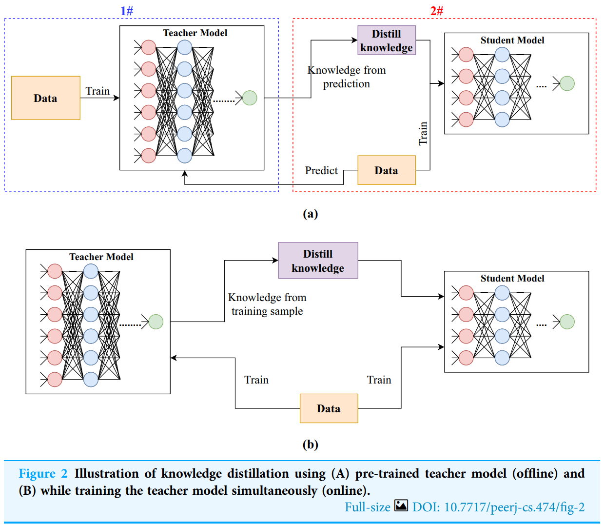
For details on the different methods, see Distilling the Knowledge in a Neural Network, Google, Knowledge distillation in deep learning and its applications, and Knowledge Distillation: A Survey.
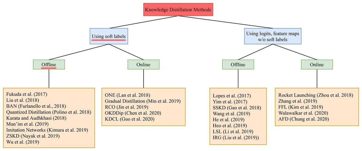
An illustration of the different categories of knowledge distillation methods, and of the branches within each category. In this section, we implement offline distillation using soft labels, underlined in red in the picture. Adapted from Knowledge distillation in deep learning and its applications.
Implementing offline distillation with soft labels
The teacher is a pre-trained model, and the student a smaller one, e.g., with fewer layers and a smaller embedding. The teacher is frozen: it runs in evaluation mode (no dropout), and its forward pass runs inside torch.no_grad(), so that no computation graph or gradients are created for it. At every training step, both models process the same batch, and the student learns to match the teacher’s output distribution at every position of the sequence. We compute the teacher’s soft labels on the fly instead of storing them on disk: storing them takes batch size × sequence length × vocabulary size values per batch, and only pays off when the teacher is too large to run next to the student (in that case, one usually stores only the top-k logits, together with the inputs they belong to).
The loss is the Kullback-Leibler (KL) divergence between the teacher’s distribution \(p\) and the student’s distribution \(q\):
\[\begin{equation} \begin{split} D_{KL}(p \parallel q) & = H(p,q) - H(p) \\ & = - \sum_i p_i \log (q_i) + \sum_i p_i \log (p_i) \\ & = \sum_i p_i \log \frac{p_i}{q_i} \end{split} \end{equation}\]where \(H(p,q)\) is the cross entropy and \(H(p)\) the entropy of the teacher’s distribution. Since \(H(p)\) does not depend on the student, minimizing the KL divergence is equivalent to minimizing the cross entropy. The loss values differ, though: the KL divergence is zero when both distributions match, while the cross entropy equals the entropy of the target. This is why the cross entropy is the usual loss for hard labels, whose entropy is zero, and the KL divergence is used to compare two distributions. In PyTorch, F.kl_div expects the student’s log-probabilities as input. We also pass the teacher’s distribution as log-probabilities (log_target=True), which the documentation recommends to avoid numerical issues. We flatten the logits to shape (batch × sequence length, vocabulary size) and use reduction='batchmean', so that the loss is the mean KL divergence per token.
The temperature \(t\) controls how soft the distributions are. For logits \(z\), the softened output is:
\[y_i (x \mid t) = \frac{ \exp\frac{z_i(x)}{t} }{ \sum_j \, \exp\frac{z_j(x)}{t} }\]A temperature above 1 flattens the distribution and reveals the relative probabilities of the unlikely tokens, which carry most of the extra information. Since the gradients of the softened loss scale with \(1/t^2\), we multiply the loss by \(t^2\), as proposed by Hinton et al., so that the size of the gradients does not depend on the temperature. A common variant adds the regular cross entropy with the ground-truth labels, weighted by a factor \(\alpha\). There are also claims that the mean squared error between logits works better than the KL divergence (Kim et al.). For LLMs, recent methods also train the student on sequences it generated itself, scored by the teacher (on-policy distillation), which removes the mismatch between the sequences seen in training and in generation.
The following code implements the distillation loss, and a training step of the student:
Show code
def distillation_loss(logits_student, logits_teacher, temperature):
    """ KL divergence between the softened distributions of the teacher and the student, averaged per token, and
        scaled by temperature^2 so that the size of the gradients does not depend on the temperature.
        logits_student, logits_teacher: [B, S, V] """
    V = logits_student.size(-1)
    log_p_student = F.log_softmax(logits_student.reshape(-1, V) / temperature, dim=-1)  # [B, S, V] -> [B*S, V]
    log_p_teacher = F.log_softmax(logits_teacher.reshape(-1, V) / temperature, dim=-1)  # [B, S, V] -> [B*S, V]
    return F.kl_div(log_p_student, log_p_teacher, log_target=True, reduction='batchmean') * temperature ** 2


def distillation_step(student, teacher, tokens, optimizer, temperature=2.0):
    """ One training step of the student on a batch of tokens: [B, S]. The teacher is frozen, in evaluation mode, and
        runs without gradients. student(tokens) and teacher(tokens) return the logits: [B, S, V] and a KV cache """
    student.train()
    logits_student, _ = student(tokens)
    with torch.no_grad():
        logits_teacher, _ = teacher(tokens)
    loss = distillation_loss(logits_student, logits_teacher, temperature)
    loss.backward()
    torch.nn.utils.clip_grad_norm_(student.parameters(), max_norm=1.0)  # against exploding gradients
    optimizer.step()
    optimizer.zero_grad(set_to_none=True)  # sets the gradients to None instead of 0, to save memory
    return loss.item()


# usage, with a pre-trained teacher and a smaller student:
# teacher.eval()
# optimizer = torch.optim.Adam(student.parameters(), lr=lr)
# for tokens in batches:
#     loss = distillation_step(student, teacher, tokens, optimizer)
Speculative decoding: more than one token per forward pass
The idea
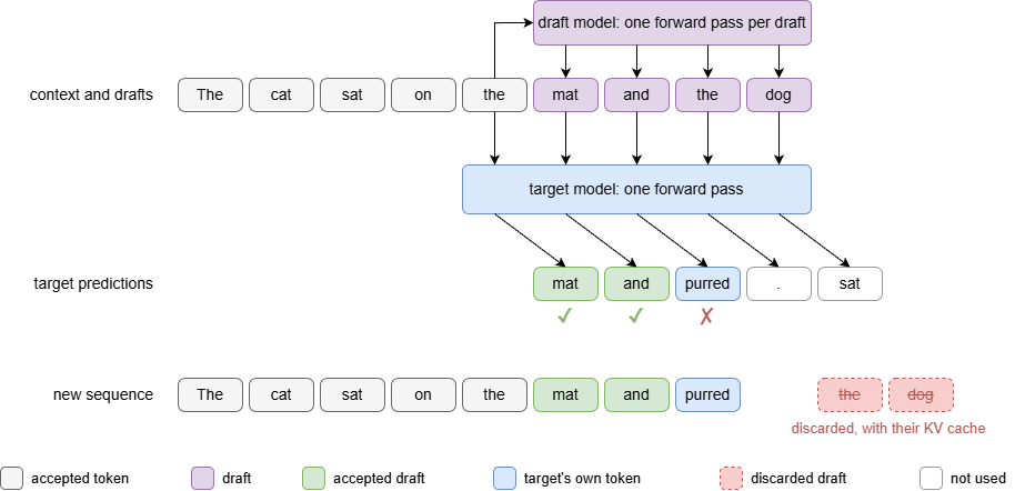
Decode is memory-bound: a forward pass over one token costs about the same as a forward pass over a handful of tokens, because the time goes into reading the weights. Speculative decoding exploits this. A cheap method drafts \(K\) tokens, and the large target model checks all of them in a single forward pass. Every draft token the target agrees with is a token generated almost for free. When the target disagrees, we keep the tokens before the disagreement, take the target’s own token at the disagreement, and draft again. With the right acceptance rule, the output is exactly the same as with the target model alone: speculative decoding is lossless.
If each draft token is accepted independently with probability \(\alpha\), the expected number of tokens produced per forward pass of the target model, including the target’s own token after the last accepted draft, is:
\[\frac{1 - \alpha^{K+1}}{1 - \alpha}\]Drafting is not free. If drafting one token costs a fraction \(c\) of a forward pass of the target, and a verification costs about as much as a regular decoding step (decode is memory-bound), the expected speedup over decoding with the target alone is (Leviathan et al.):
\[\frac{1 - \alpha^{K+1}}{(1 - \alpha)(cK + 1)}\]The speedup therefore depends on how often the drafts are right and on how cheap they are. Speculative decoding helps most at small batch sizes, where decode is most memory-bound; at large batch sizes, the GPU is already busy, and the extra verification work competes with useful work. The methods below differ in where the drafts come from.
Draft-model speculative decoding
The original method (Leviathan et al., Chen et al.) drafts with a small language model that uses the same tokenizer as the target, ideally a distilled version of the target, such as the student of the distillation section above. Each iteration:
- the draft model generates \(K\) tokens autoregressively;
- the target model runs one forward pass over the context and the \(K\) draft tokens, which gives its distribution at each of the \(K\) draft positions, plus one more after the last draft;
- the draft tokens are checked from left to right.
The acceptance rule depends on how we decode.
With greedy decoding, draft tokens are accepted while they are equal to the target’s most likely token. At the first mismatch, the draft token is replaced by the target’s most likely token, and the remaining drafts are discarded. If all \(K\) drafts are accepted, the target’s prediction after the last draft is appended as a bonus token. The output is identical to greedy decoding with the target alone.
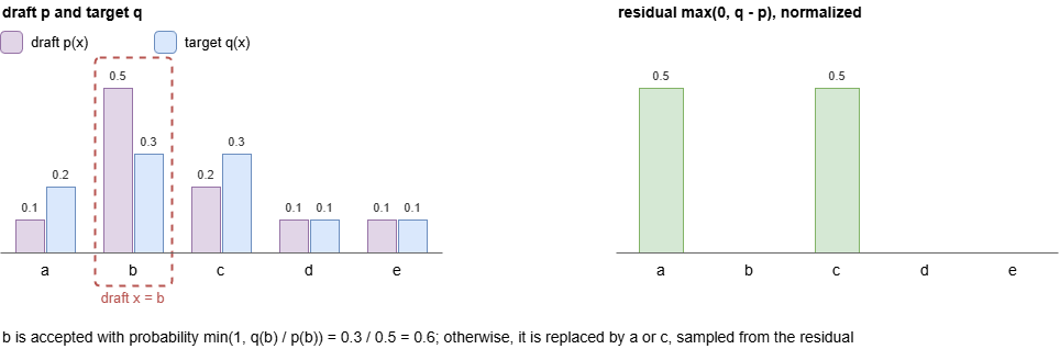
With sampling (speculative sampling), the draft model samples each token \(x\) from its distribution \(p\), and the target accepts it with probability \(\min\left(1, q(x) / p(x)\right)\), where \(q\) is the target’s distribution. On rejection, a replacement token is sampled from the normalized residual distribution \(\max(0, q - p)\), and the remaining drafts are discarded. This modified rejection sampling produces tokens distributed exactly as \(q\), and if all \(K\) drafts are accepted, a bonus token is sampled from the target’s distribution after the last draft. The rule holds for any \(p\), as long as it is the distribution the drafts were actually sampled from. Greedy drafts are the special case of a one-hot \(p\): the target accepts the draft \(x\) with probability \(q(x)\), and on rejection samples from \(q\) without \(x\), which still yields tokens distributed as \(q\). What breaks the guarantee is drafting greedily while using the draft model’s softmax probabilities as \(p\).
In a batch, each sequence accepts a different number of tokens, so the sequences progress at different speeds, and engines track their lengths separately, as in continuous batching.
To keep it simple, the following code generates one sequence at a time, and the whole sequence must fit in the context window. Both models use a KV cache: after each verification, the cache of the target is truncated to the accepted tokens, and the draft model reuses the part of its own cache that is still valid.
The following code implements greedy speculative decoding with a draft model, and gives the same output as greedy decoding with the target alone:
Show code
def truncate_cache(kv_cache, n):
    """ Keeps the first n tokens of a KV cache: a list with a tuple of tensors per layer, such as the keys and the
        values: [B, H, P, h], with the tokens in dimension 2 """
    return [tuple(t[:, :, :n] for t in layer_cache) for layer_cache in kv_cache]


def generate_speculative(model, prompt, n_tokens, propose, n_drafts):
    """ Greedy speculative decoding of a single sequence, prompt: [1, S]. model(tokens, kv_cache) returns the logits of
        the new tokens: [1, S, V] and the KV cache with them appended. At every iteration, propose(tokens, k) returns
        up to k draft tokens: [1, k], and the target checks all of them in a single forward pass. The cache of the
        target holds all the accepted tokens except the last one, which is processed together with the drafts. The
        whole sequence must fit in the context window """
    n_total = prompt.size(1) + n_tokens
    tokens, kv_cache = prompt, None
    if prompt.size(1) > 1:
        _, kv_cache = model(prompt[:, :-1])
    while tokens.size(1) < n_total:
        drafts = propose(tokens, min(n_drafts, n_total - tokens.size(1) - 1))  # [1, k]

        # predictions of the target after the last accepted token and after each draft: [1, k+1, V] -> [1, k+1]
        logits, kv_cache = model(torch.cat([tokens[:, -1:], drafts], dim=1), kv_cache)
        predictions = logits.argmax(dim=-1)

        # accept the drafts while they match the predictions of the target
        n_accepted = 0
        while n_accepted < drafts.size(1) and drafts[0, n_accepted] == predictions[0, n_accepted]:
            n_accepted += 1

        # keep the accepted drafts, plus the target's own token at the first mismatch (or the bonus token, after the
        # last draft if all were accepted), and drop the cache entries of the rejected drafts
        tokens = torch.cat([tokens, drafts[:, :n_accepted], predictions[:, n_accepted:n_accepted + 1]], dim=1)
        kv_cache = truncate_cache(kv_cache, tokens.size(1) - 1)
    return tokens  # [1, S + n_tokens]


class DraftModel:
    """ Proposes greedy drafts with a small model, model(tokens, kv_cache) -> (logits, kv_cache), and its own KV cache.
        On every call, it reuses the cache of the longest prefix of the tokens it has already processed """

    def __init__(self, model):
        self.model = model
        self.kv_cache, self.processed = None, None  # the cache, and the tokens it holds: [1, P]

    def __call__(self, tokens, n_drafts):
        if n_drafts == 0:
            return tokens[:, :0]

        # number of leading tokens processed before and still valid; the last token is always processed, to predict
        # the first draft
        n_cached = 0
        if self.processed is not None:
            n = min(self.processed.size(1), tokens.size(1) - 1)
            mismatches = (self.processed[0, :n] != tokens[0, :n]).nonzero()
            n_cached = mismatches[0].item() if len(mismatches) > 0 else n
        kv_cache = truncate_cache(self.kv_cache, n_cached) if n_cached > 0 else None

        new_tokens, drafts = tokens[:, n_cached:], []
        for _ in range(n_drafts):  # greedy generation with the draft model
            logits, kv_cache = self.model(new_tokens, kv_cache)  # [1, S, V]
            new_tokens = logits[:, -1:].argmax(dim=-1)            # [1, 1]
            drafts.append(new_tokens)
        self.kv_cache = kv_cache
        self.processed = torch.cat([tokens] + drafts[:-1], dim=1)  # the last draft was not processed
        return torch.cat(drafts, dim=1)                             # [1, n_drafts]


# usage, with a small model that uses the same tokenizer as the target:
# tokens = generate_speculative(target, prompt, n_tokens, DraftModel(draft), n_drafts=4)
The following code implements the acceptance rule of speculative sampling, which replaces the greedy acceptance in the loop above:
Show code
def accept_sampling(drafts, p, q):
    """ Speculative sampling: verifies the drafts: [k], sampled from the distributions p: [k, V] of the draft model,
        with the distributions q: [k+1, V] of the target after the last accepted token and after each draft. A draft
        x is accepted with probability min(1, q(x) / p(x)). Returns the accepted drafts, followed by a token sampled
        from the residual max(0, q - p) at the first rejection, or by a bonus token sampled from the last q if all the
        drafts are accepted """
    for i, x in enumerate(drafts.tolist()):
        if torch.rand(()) >= q[i, x] / p[i, x]:  # rejected
            residual = (q[i] - p[i]).clamp(min=0)  # [V]
            return torch.cat([drafts[:i], torch.multinomial(residual / residual.sum(), 1)])
    return torch.cat([drafts, torch.multinomial(q[-1], 1)])


# in generate_speculative, the drafter samples the drafts and returns their distributions p, the distributions of
# the target are q = softmax(logits / temperature), and accept_sampling replaces the greedy acceptance
Prompt lookup decoding
Prompt lookup decoding needs no draft model at all. It takes the last few generated tokens (an n-gram), searches for the same n-gram earlier in the prompt or in the generated text, and proposes the tokens that followed it as drafts; the verification is the same as above. It costs almost nothing, and gives large speedups when the output copies from the input, as in summarization, code editing, question answering over documents, or rewriting a previous answer. Related methods draft from other sources: lookahead decoding collects n-grams from Jacobi iterations of the model itself, and REST retrieves continuations from a datastore of text.
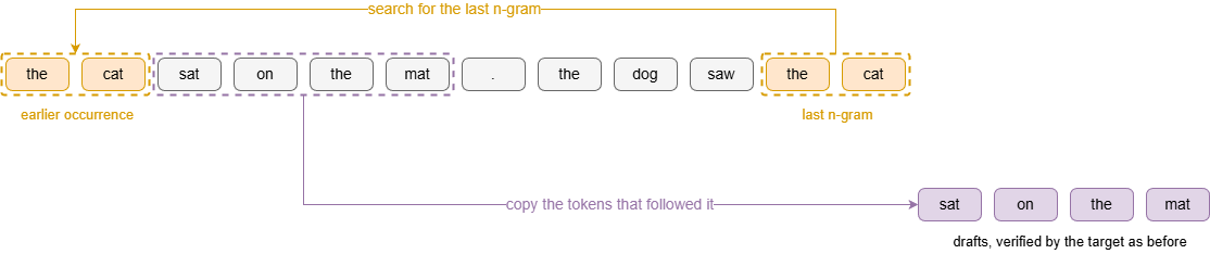
The following code implements prompt lookup decoding. It reuses the verification loop of speculative decoding, with a different source of drafts:
Show code
def prompt_lookup(tokens, n_drafts, max_ngram=3):
    """ Drafts the tokens that followed the most recent earlier occurrence of the last n-gram of the sequence, trying
        the longest n-grams first. tokens: [1, S] -> drafts: [1, k], with k <= n_drafts, and k = 0 if the n-gram never
        occurred before """
    sequence = tokens[0]  # [S]
    for n in range(max_ngram, 0, -1):
        if sequence.size(0) <= n:
            continue
        ngram = sequence[-n:]                     # [n]
        windows = sequence[:-1].unfold(0, n, 1)  # the earlier n-grams: [S-n, n]
        matches = (windows == ngram).all(dim=1).nonzero()
        if len(matches) > 0:
            start = matches[-1].item() + n  # first token after the most recent match
            return sequence[start:start + n_drafts].unsqueeze(0)
    return tokens[:, :0]


# usage: the verification loop of speculative decoding, with a different source of drafts
# tokens = generate_speculative(model, prompt, n_tokens, prompt_lookup, n_drafts=4)
Medusa
Medusa adds a few extra decoding heads on top of the last hidden state of the target model: the original output head predicts the next token, and head \(i\) predicts the token \(i+1\) positions ahead. The top candidates of each head are combined into a tree of possible continuations, and all of them are verified in a single forward pass with tree attention, a mask that lets each candidate attend only to its own ancestors in the tree. The longest accepted path is kept. Training only the heads, with the model frozen (Medusa-1), gives speedups above 2.2 times; training the heads together with the model (Medusa-2) reaches 2.3 to 3.6 times. Medusa needs no separate draft model, but each head guesses its token independently, without seeing the tokens guessed by the other heads, so the accuracy drops quickly for later positions. For sampling, Medusa also proposes a faster typical acceptance rule, which is not exactly lossless.

The following code implements the Medusa heads, the tree of candidates and its attention mask, and one step of greedy decoding, which keeps only the KV cache of the accepted path:
Show code
class MedusaHeads(nn.Module):
    """ Medusa decoding heads, on the last hidden states of the target: head k predicts the token k positions after the
        next one, with a residual block that starts as the identity (zero weights) and a copy of the output layer of
        the target: logits_k = W_k (SiLU(W1_k h) + h) """

    def __init__(self, lm_head, num_heads=4):
        super().__init__()
        E, V = lm_head.in_features, lm_head.out_features
        self.blocks = nn.ModuleList(nn.Linear(E, E) for _ in range(num_heads))
        self.heads = nn.ModuleList(nn.Linear(E, V, bias=lm_head.bias is not None) for _ in range(num_heads))
        for block, head in zip(self.blocks, self.heads):
            nn.init.zeros_(block.weight)
            nn.init.zeros_(block.bias)
            head.load_state_dict(lm_head.state_dict())

    def forward(self, h):
        """ h: [B, S, E] -> logits of the num_heads tokens after the next one: [B, S, num_heads, V] """
        return torch.stack([head(F.silu(block(h)) + h) for block, head in zip(self.blocks, self.heads)], dim=2)


def medusa_tree(next_token, head_logits, top_k=2):
    """ Tree of candidate continuations: the target's next token at the root, the top_k tokens of head 1 as its
        children, the top_k tokens of head 2 as the children of each of them, and so on. head_logits: [num_heads, V],
        at the last accepted token. Returns the tokens of the N nodes: [N], the parent of each node (-1 for the root,
        parents before children) and the depth of each node: [N] """
    tokens, parents, depths, level = [next_token], [-1], [0], [0]  # level: the nodes of the deepest level so far
    for depth, logits in enumerate(head_logits, start=1):
        top = logits.topk(top_k).indices.tolist()
        new_level = []
        for parent in level:
            for token in top:
                new_level.append(len(tokens))
                tokens.append(token)
                parents.append(parent)
                depths.append(depth)
        level = new_level
    return torch.tensor(tokens), parents, torch.tensor(depths)


def tree_attention_mask(parents):
    """ Tree attention: [N, N], True where node i can attend to node j, i.e. j is i or one of its ancestors """
    mask = torch.eye(len(parents), dtype=torch.bool)
    for i, parent in enumerate(parents):
        if parent >= 0:
            mask[i] |= mask[parent]  # the row of the parent already holds its ancestors
    return mask


def longest_accepted_path(tokens, parents, predictions):
    """ Greedy verification of the tree: the root is the target's own token, and a node is accepted if its parent is
        accepted and its token is the target's prediction after its parent. tokens, predictions: lists of N tokens.
        Returns the nodes of the longest accepted path, from the root """
    paths = {0: [0]}  # path from the root to every accepted node
    for i in range(1, len(parents)):
        if parents[i] in paths and tokens[i] == predictions[parents[i]]:
            paths[i] = paths[parents[i]] + [i]
    return max(paths.values(), key=len)


def medusa_step(model, heads, tokens, kv_cache, next_token, head_logits, top_k=2):
    """ One step of greedy decoding with Medusa. tokens: [1, T], the accepted tokens, all in the KV cache; next_token:
        the target's next token; head_logits: [num_heads, V], of the Medusa heads at the last accepted token.
        model(tokens, kv_cache, mask, positions) returns the logits [1, N, V] and the last hidden states [1, N, E] of
        the new tokens, and the cache with them appended """
    tree, parents, depths = medusa_tree(next_token, head_logits, top_k)  # [N]
    T, device = tokens.size(1), tokens.device

    # one forward pass over the tree: every node sees the cached tokens and its ancestors, at the position after its
    # parent: mask [N, T+N]
    mask = torch.cat([torch.ones(len(tree), T, dtype=torch.bool), tree_attention_mask(parents)], dim=1)
    logits, hidden, kv_cache = model(tree[None].to(device), kv_cache, mask.to(device), (T + depths).to(device))
    path = longest_accepted_path(tree.tolist(), parents, logits[0].argmax(dim=-1).tolist())

    # keep the accepted path, and its entries in the cache
    keep = torch.tensor(list(range(T)) + [T + i for i in path], device=device)
    kv_cache = [tuple(t[:, :, keep] for t in layer_cache) for layer_cache in kv_cache]
    tokens = torch.cat([tokens, tree[path][None].to(device)], dim=1)

    # the target's token after the path, and the Medusa heads at the last node of the path, for the next step
    next_token = logits[0, path[-1]].argmax().item()
    head_logits = heads(hidden[:, path[-1]:path[-1] + 1])[0, 0]  # [num_heads, V]
    return tokens, kv_cache, next_token, head_logits


# usage: prefill the prompt: [1, S], with the causal_mask of the post on attention, then run medusa_step:
# logits, hidden, kv_cache = model(prompt, None, causal_mask(S, S), torch.arange(S))
# tokens, next_token, head_logits = prompt, logits[0, -1].argmax().item(), heads(hidden[:, -1:])[0, 0]
# while tokens.size(1) < S + n_tokens:
#     tokens, kv_cache, next_token, head_logits = medusa_step(model, heads, tokens, kv_cache, next_token, head_logits)
EAGLE
EAGLE drafts at the level of features rather than tokens. Its draft model is a single lightweight transformer layer that takes the top-layer hidden states (features) of the target, together with the embeddings of the tokens sampled so far, predicts the next feature, and turns it into a token with the target’s own output layer. Feature sequences are more regular than token sequences, so these drafts are much more accurate than Medusa’s independent heads. EAGLE-2 shapes the draft tree dynamically, expanding the branches where the draft model is confident. EAGLE-3 (NeurIPS 2025) noticed that EAGLE barely improved with more training data, and traced this to its feature prediction objective. It drops feature prediction and predicts tokens directly, fuses low-, mid- and high-level features of the target instead of the top layer only, and uses training-time test: during training, the draft model is fed its own predictions, to simulate multi-step drafting. EAGLE-3 reaches speedups of up to 6.5 times, about 1.4 times more than EAGLE-2, and 1.38 times higher throughput at a batch size of 64 in SGLang. EAGLE-style drafting is supported by vLLM, SGLang and TensorRT-LLM.
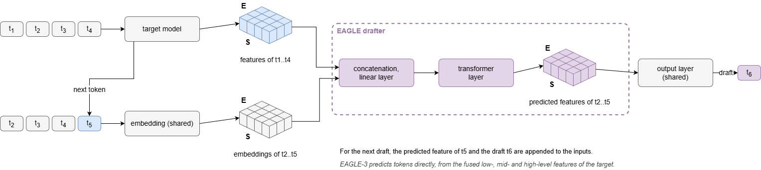
The following code implements an EAGLE drafter, and a drafting loop that the MTP modules below also use:
Show code
class EagleDrafter(nn.Module):
    """ EAGLE drafter: a transformer block predicts the next feature (last hidden state) of the target from its
        features and the embeddings of the tokens one position ahead, and the output layer of the target turns the
        predicted features into tokens. embedding and lm_head are those of the target, frozen; block: a transformer
        block with causal attention, block(x, kv_cache=None) -> (x, kv_cache). EAGLE-3 predicts tokens directly, from
        the concatenated features of a low, a middle and a high layer of the target """

    def __init__(self, embedding, lm_head, block):
        super().__init__()
        E = embedding.embedding_dim
        self.embedding, self.lm_head, self.block = embedding, lm_head, block
        self.fc = nn.Linear(2 * E, E)

    def forward(self, features, tokens):
        """ features: [B, S, E] at positions 1..S, tokens: [B, S] at positions 2..S+1 -> predicted features at positions
            2..S+1: [B, S, E], and logits of the tokens at positions 3..S+2: [B, S, V] """
        x = self.fc(torch.cat([features, self.embedding(tokens)], dim=-1))  # [B, S, 2E] -> [B, S, E]
        features, _ = self.block(x)                                         # [B, S, E]
        return features, self.lm_head(features)


@torch.no_grad()
def draft_with_features(drafter, features, tokens, n_drafts):
    """ Drafts n_drafts tokens with a drafter that predicts features: an EAGLE drafter, or an MTP module (below).
        features: [1, S, E], the target's features of the tokens 1..S; tokens: [1, S], the tokens 2..S+1, the last one
        being the last accepted token. Every draft appends its predicted feature and its token. For simplicity, the
        drafter recomputes the whole sequence at every draft, instead of using a KV cache """
    drafts = tokens[:, :0]
    for _ in range(n_drafts):
        predicted, logits = drafter(features, tokens)  # [1, S, E], [1, S, V]
        draft = logits[:, -1:].argmax(dim=-1)           # [1, 1]
        features = torch.cat([features, predicted[:, -1:]], dim=1)
        tokens = torch.cat([tokens, draft], dim=1)
        drafts = torch.cat([drafts, draft], dim=1)
    return drafts                                       # [1, n_drafts]


# usage, with features(tokens) the target's features of the tokens, kept from its forward passes:
# propose = lambda tokens, k: draft_with_features(drafter, features(tokens[:, :-1]), tokens[:, 1:], k)
# tokens = generate_speculative(target, prompt, n_tokens, propose, n_drafts=4)
DFlash
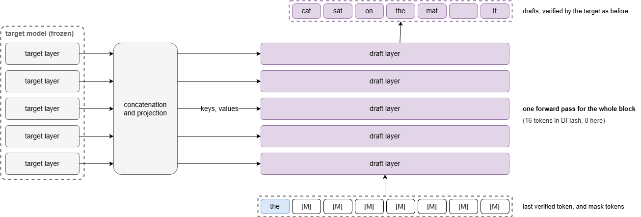
DFlash (Chen, Liang and Liu, UC San Diego, ICML 2026) replaces the autoregressive drafter with a small block diffusion model. Autoregressive drafters such as EAGLE-3 need one forward pass per drafted token, so they are kept very shallow (a single transformer layer for EAGLE-3), which, according to the authors, limits their acceptance length and keeps practical speedups around 2-3 times. DFlash instead takes the last verified token, appends 15 mask tokens, and fills the whole block in a single forward pass, so its drafting cost barely grows with the block size (in the speedup formula above, \(cK\) becomes about \(c\)) and it can afford a deeper drafter: a 5-layer DFlash fills a 16-token block faster than a 1-layer EAGLE-3 drafts 8 tokens, and gets more of them accepted.
A drafter this small predicts poorly on its own (without target features, a 5-layer diffusion drafter only reaches about 3 times), so DFlash conditions it on the target: the hidden states of 5 target layers, spread from shallow to deep, are concatenated, projected, and injected into the keys and values of every draft layer, instead of only into the drafter’s input as in EAGLE-3, so the acceptance length keeps improving as draft layers are added. The drafter reuses the target’s frozen embedding and output head, and only its transformer layers are trained, on responses generated by the target: each training block starts at a randomly sampled anchor token, as at inference, all blocks of a sequence are trained in one pass with a block-sparse attention mask, and the loss favors early positions, since one early mistake invalidates the rest of the block. Verification is unchanged, so the output stays lossless. Each round verifies a single drafted block, not a tree: DDTree builds a draft tree from the per-position predictions of the DFlash drafter, and verifies it with tree attention.
On Qwen3-8B with greedy decoding, the paper reports about 6.5 tokens committed per verification step on average and up to 6.1 times faster decoding than the baseline, about 2.5 times the speedup of EAGLE-3, with the largest gains on math and code and the smallest on open-ended chat (about 2.8 times). In SGLang on a B200, the speedup drops from about 4-5 times for a single request to about 2.5-3 times at 32 concurrent requests, as verifying 16-token blocks becomes compute-bound. Drafters trained on 4K-token contexts also lose acceptance on longer inputs, which a short long-context fine-tune recovers. Unlike multi-token prediction (below), which only helps models pre-trained with MTP modules, a DFlash drafter is trained after the fact against a frozen target, so it can be added to almost any model. However, at the time of writing its training recipe is not public, so in practice one uses the drafters released by z-lab, for Qwen3.5/3.6, gpt-oss, Gemma 4 and Kimi K2.5, among others. DFlash runs in vLLM and SGLang, with an MLX version for Apple Silicon.
Self-speculative decoding: LayerSkip
LayerSkip uses the early layers of the target model as the draft. The model is trained with layer dropout, which skips the later layers more often, and with an early exit loss, which trains every layer to make good predictions through the shared output head. At inference, the draft exits after the first \(E\) layers, and the verification runs only the remaining layers, reusing the computation and the cache of the first \(E\). There is no second model to store, and the reported speedups reach up to about 2 times on summarization and coding tasks.
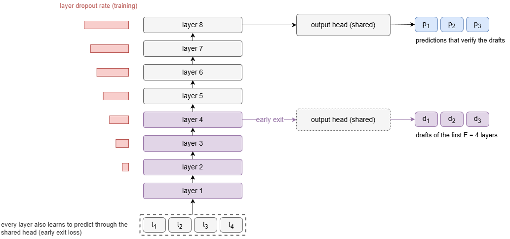
The following code implements a simplified LayerSkip: the early exit loss with layer dropout for training, and drafting with the first layers at inference:
Show code
class LayerSkip(nn.Module):
    """ LayerSkip, simplified: a decoder whose layers can exit early, through the shared output head (final norm and
        output layer). In training, layer dropout skips layer l of each sequence with a probability that grows with
        depth, and the early exit loss trains every layer to predict the next token. At inference, the first layers
        draft and all the layers verify. embedding(tokens, start): token and positional embeddings of the tokens at
        positions start, start+1, ...; blocks: transformer blocks with causal attention,
        block(x, kv_cache=None) -> (x, kv_cache) """

    def __init__(self, embedding, blocks, norm, head, p_max=0.2):
        super().__init__()
        self.embedding, self.blocks, self.norm, self.head = embedding, nn.ModuleList(blocks), norm, head
        self.p_max = p_max  # layer dropout rate of the last layer

    def forward(self, tokens, kv_cache=None, exit_layer=None):
        """ tokens: [1, S], the new tokens -> logits after the first exit_layer layers (all by default): [1, S, V], and
            the KV cache of these layers, with the new tokens appended """
        blocks = self.blocks[:exit_layer]
        kv_cache = kv_cache or [None] * len(blocks)
        start = 0 if kv_cache[0] is None else kv_cache[0][0].size(2)  # number of cached tokens
        x = self.embedding(tokens, start)                              # [1, S, E]
        new_cache = []
        for block, layer_cache in zip(blocks, kv_cache):
            x, layer_cache = block(x, kv_cache=layer_cache)
            new_cache.append(layer_cache)
        return self.head(self.norm(x)), new_cache

    def loss(self, tokens, targets):
        """ Early exit loss with layer dropout: the cross-entropy of every layer through the shared output head,
            averaged with weights that grow with depth. tokens, targets: [B, S] """
        x, L = self.embedding(tokens, 0), len(self.blocks)  # [B, S, E]
        loss = 0.0
        for l, block in enumerate(self.blocks):
            p = self.p_max * l / max(L - 1, 1) if self.training else 0.0
            keep = torch.rand(x.size(0), 1, 1, device=x.device) >= p  # layer dropout, per sequence: [B, 1, 1]
            x = torch.where(keep, block(x)[0], x)
            logits = self.head(self.norm(x))                           # [B, S, V]
            loss = loss + (l + 1) * F.cross_entropy(logits.flatten(0, 1), targets.flatten())
        return loss / (L * (L + 1) / 2)


# usage: the first layers draft and the whole model verifies. LayerSkip also reuses the KV cache and the hidden states
# of the first layers in the verification, which this sketch recomputes
# early_exit = lambda tokens, kv_cache: model(tokens, kv_cache, exit_layer=4)
# tokens = generate_speculative(model, prompt, n_tokens, DraftModel(early_exit), n_drafts=4)
Multi-token prediction
Multi-token prediction (MTP) trains the model itself, during pre-training, to predict several future tokens at every position, instead of only the next one. This has two benefits. During training, every position gets a denser learning signal, which can improve the representations learned by the model. At inference, the extra predictions are drafts: the model drafts for itself, without a separate draft model, and the verification is the same as in speculative decoding.
Parallel heads
Gloeckle et al. (Meta, 2024) add \(n\) output heads on top of a shared trunk. The trunk \(f_s\) computes a representation \(z_t = f_s(x_{1:t})\) of the context, and head \(i\), a transformer layer \(f_{h_i}\) followed by the unembedding \(f_u\) shared by all heads, predicts the token \(i\) positions ahead:
\[P_\theta(x_{t+i} \mid x_{1:t}) = \text{softmax}\left( f_u \left( f_{h_i} ( z_t ) \right) \right)\]The training loss sums the cross-entropy losses of the \(n\) heads:
\[L_n = - \sum_t \sum_{i=1}^{n} \log P_\theta(x_{t+i} \mid x_{1:t})\]As the vocabulary is large, holding the logits of all heads at once would dominate the memory of training. Instead, after the forward pass of the trunk, the forward and backward passes of the heads run one after the other, accumulating their gradients at the output of the trunk, so that only the logits of one head are in memory at a time. The benefits grow with the model size, and small models can even get worse: the 13B model of the paper solves 12% more problems on HumanEval and 17% more on MBPP than a comparable next-token model. At inference, the extra heads are drafts for self-speculative decoding, making a model trained to predict 4 tokens up to 3 times faster. However, as in Medusa, each head predicts its token without seeing the tokens predicted by the other heads.
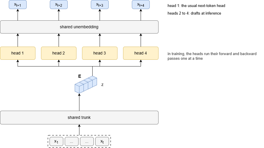
The following code implements the parallel heads, and the backward pass that keeps the logits of only one head in memory:
Show code
class MultiTokenHeads(nn.Module):
    """ Multi-token prediction with parallel heads (Gloeckle et al.): head i, a transformer block followed by the output
        layer shared by all heads (final norm and unembedding), predicts the token i positions ahead from the output z
        of the trunk. Head 1 is the usual next-token head. blocks: transformer blocks with causal attention,
        block(x, kv_cache=None) -> (x, kv_cache) """

    def __init__(self, blocks, unembedding):
        super().__init__()
        self.blocks, self.unembedding = nn.ModuleList(blocks), unembedding

    def forward(self, z):
        """ z: [B, S, E] -> logits of the tokens 1, 2, ..., n positions ahead: [B, S, n, V]. At inference, the heads at
            the last position draft the next n tokens, the first of which is the model's own next token """
        return torch.stack([self.unembedding(block(z)[0]) for block in self.blocks], dim=2)

    def loss_backward(self, z, tokens):
        """ Training, instead of loss.backward(): z: [B, S, E], output of the trunk for the input tokens: [B, S]. The
            forward and backward passes of the heads run one after the other, accumulating their gradients at z, so
            that only the logits of one head are in memory at a time; then the trunk runs its backward pass once.
            Returns the loss: the sum of the cross-entropy losses of the heads """
        z_heads = z.detach().requires_grad_()  # the gradients of the heads accumulate in z_heads.grad
        total = 0.0
        for i, block in enumerate(self.blocks, start=1):
            logits = self.unembedding(block(z_heads)[0][:, :-i])  # predictions of the tokens i positions ahead
            loss = F.cross_entropy(logits.flatten(0, 1), tokens[:, i:].flatten())
            loss.backward()
            total += loss.item()
        z.backward(z_heads.grad)
        return total
Sequential modules
DeepSeek-V3 predicts the extra tokens sequentially instead, keeping the complete causal chain at each prediction depth. It adds \(D\) MTP modules, where module \(k\) has its own transformer block \(\text{TRM}_k\) and projection matrix \(M_k\), and shares the embedding layer and the output head with the main model. For the token at position \(i\), module \(k\) combines the representation \(h_i^{k-1}\) of the previous depth (the output of the main model, for \(k=1\)) with the embedding of the token \(t_{i+k}\):
\[h_i^{\prime k} = M_k \left[ \text{RMSNorm}(h_i^{k-1}) ; \text{RMSNorm}(\text{Emb}(t_{i+k})) \right]\]runs it through its transformer block, \(h^{k} = \text{TRM}_k(h^{\prime k})\), and predicts the token \(t_{i+k+1}\) with the shared output head, \(P^{k}_{i+k+1} = \text{OutHead}(h^{k}_i)\). Each depth has its own cross-entropy loss \(L^k_\text{MTP}\), and their average is added to the main next-token loss with a weight \(\lambda\):
\[L_\text{MTP} = \frac{\lambda}{D} \sum_{k=1}^{D} L^k_\text{MTP}\]With \(D\) modules, the main model predicts \(t_{i+1}\); module 1 combines its hidden state with the embedding of \(t_{i+1}\) to predict \(t_{i+2}\); module 2 combines the hidden state of module 1 with the embedding of \(t_{i+2}\) to predict \(t_{i+3}\); and so on. Each prediction thus depends on the tokens before it, unlike the parallel heads of Gloeckle et al., which predict their tokens independently. Besides the shared embedding and output head, each module only adds its projection matrix and its transformer block. DeepSeek-V3 uses a single module (\(D=1\)), with \(\lambda = 0.3\) for the first 10T training tokens and \(0.1\) for the remaining 4.8T, and its published MTP weights add 14B parameters to the 671B of the main model.
The authors report better results on most benchmarks, and suggest that MTP may make the model pre-plan its representations for better predictions of future tokens. At inference, the module can be discarded, and the model runs as a regular next-token model, or used as a draft: the second predicted token is accepted 85-90% of the time, giving 1.8 times more tokens per second. Note that an MTP module is very close to an EAGLE draft layer: both combine the features of the target with the embedding of the next token, run one transformer layer, and predict with the target’s output head. The difference is that the MTP module is trained together with the model, during pre-training.
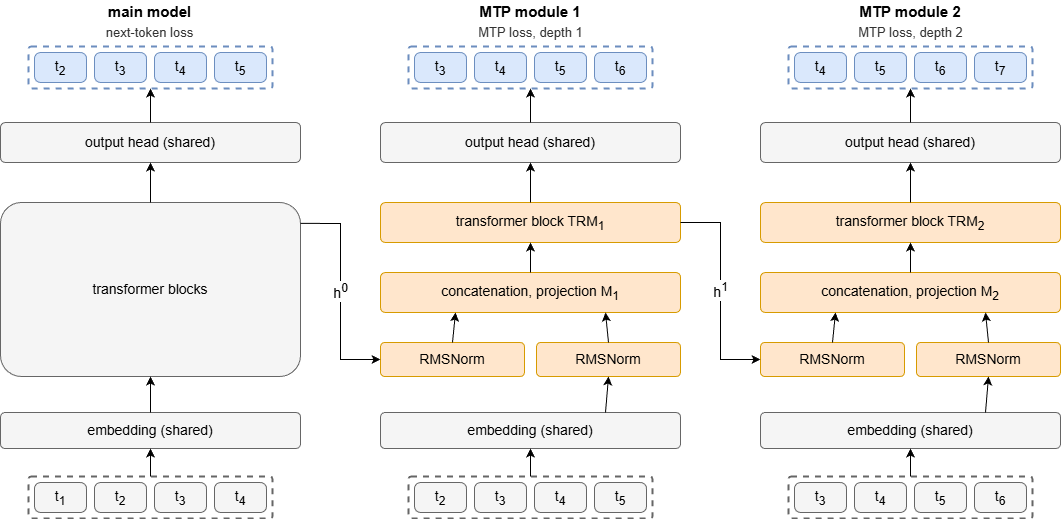
The following code implements the MTP modules of DeepSeek-V3 and their loss:
Show code
class MTPModule(nn.Module):
    """ DeepSeek-V3 multi-token prediction module k: combines the hidden states of depth k-1 (the output of the main
        model, for k = 1) with the embeddings of the tokens k positions ahead, runs its transformer block, and predicts
        the tokens k+1 positions ahead. embedding and out_head (final norm and output layer) are shared with the main
        model; block: a transformer block with causal attention, block(x, kv_cache=None) -> (x, kv_cache) """

    def __init__(self, embedding, block, out_head):
        super().__init__()
        E = embedding.embedding_dim
        self.embedding, self.block, self.out_head = embedding, block, out_head
        self.norm_h, self.norm_e = nn.RMSNorm(E), nn.RMSNorm(E)
        self.proj = nn.Linear(2 * E, E, bias=False)  # M_k

    def forward(self, h, tokens):
        """ h: [B, S, E], hidden states of depth k-1 at positions i; tokens: [B, S] at positions i+k -> hidden states
            of depth k at positions i: [B, S, E], and logits of the tokens at positions i+k+1: [B, S, V] """
        x = self.proj(torch.cat([self.norm_h(h), self.norm_e(self.embedding(tokens))], dim=-1))  # [B, S, E]
        h, _ = self.block(x)
        return h, self.out_head(h)


def mtp_loss(modules, h, tokens, lam=0.3):
    """ DeepSeek-V3 MTP loss, added to the next-token loss of the main model. h: [B, T, E], output of the main model
        for the input tokens: [B, T]. Module k predicts the tokens k+1 positions ahead, and the average of the
        cross-entropy losses of the modules is weighted by lam """
    losses = []
    for k, module in enumerate(modules, start=1):
        h, logits = module(h[:, :-1], tokens[:, k:])  # positions i = 0, ..., T-k-1: [B, T-k, E], [B, T-k, V]
        losses.append(F.cross_entropy(logits[:, :-1].flatten(0, 1), tokens[:, k + 1:].flatten()))
    return lam * sum(losses) / len(losses)


# drafting with an MTP module, run again on its own outputs for more drafts, uses the drafting loop of EAGLE:
# propose = lambda tokens, k: draft_with_features(module, features(tokens[:, :-1]), tokens[:, 1:], k)
Drafting with MTP modules
With a single module, the model drafts one extra token per forward pass. To draft more tokens, inference engines run the same module again on its own output hidden state and draft token, as with EAGLE, even though it was only trained to look one token ahead, so the acceptance drops for the later drafts. SGLang serves DeepSeek-V3 and R1 this way, with their MTP module (called NextN) as the drafter: in a large-scale deployment, LMSYS reported an average acceptance length of 2.18 tokens with a 3-token MTP window, and of 2.44 tokens with a 4-token window. Other models train more modules for inference: MiMo-7B (Xiaomi) uses a single MTP layer during pre-training, as more layers did not help, and then copies it to fine-tune two more MTP layers, with the main model and the first MTP layer frozen. On AIME24, the drafts of the first MTP layer are accepted about 90% of the time, and those of the third layer more than 75%. Native MTP modules are now common in recent models, such as Qwen3-Next and Qwen3.5: vLLM uses them as drafters, and its speculators library can fine-tune them for multi-step drafting.
Medusa, EAGLE and DFlash add a drafter to an existing model, and LayerSkip trains the model so that its own early layers can draft. MTP builds the drafter in during pre-training: its drafts are cheap and accurate, and it may even improve the model, but only models pre-trained with it can use it.
Summary of speculative decoding methods
| Method | Source of the drafts | Extra training | Extra memory | Reported speedup |
|---|---|---|---|---|
| Draft model | a separate small model | none, or distilling a draft | a second model | about 2-3x |
| Prompt lookup | n-grams of the context | none | none | large on copy-heavy tasks |
| Medusa | extra heads | the heads (or joint fine-tuning) | small | 2.2-3.6x |
| EAGLE-3 | a feature-level draft layer | the draft layer | small | up to 6.5x |
| DFlash | a block-diffusion drafter conditioned on the target’s hidden states | the drafter (target frozen) | small (a few layers) | over 6x, about 2.5x EAGLE-3’s speedup |
| LayerSkip | early layers of the model | layer dropout and early exit loss, in pre-training or fine-tuning | none | up to about 2x |
| Multi-token prediction | the model’s own MTP heads (parallel) or modules (sequential) | pre-training | small (about 2% of DeepSeek-V3) | 1.8x (DeepSeek-V3) to 3x |
The reported speedups come from the respective papers, with different models, tasks and hardware, and they shrink as the batch size grows. All these methods are lossless, except Medusa with typical acceptance.