Unsupervised Learning for Association Rules and Outliers
This post continues the posts on clustering and dimensionality reduction with two other tasks of unsupervised learning, association rule mining and outlier detection, each with a short NumPy implementation.
Association Rule Mining
Association rule learning finds the items that often appear together in a database of transactions, e.g. the products that the customers of a supermarket buy together. A rule \(X \Rightarrow Y\), e.g. \(\{\text{butter}\} \Rightarrow \{\text{eggs}\}\), says that the transactions that hold the itemset \(X\) often hold the itemset \(Y\) too. For a set of transactions \(T\), the quality of a rule is measured by:
- the support of an itemset, the fraction of the transactions that contain it:
- the confidence of a rule, the fraction of the transactions with \(X\) that also contain \(Y\):
- the lift of a rule, above 1 when \(X\) and \(Y\) appear together more often than if they were independent:
The rules are mined in two steps. First, find all the frequent itemsets, whose support is at least a minimum support. Then, split each frequent itemset into the rules whose confidence is at least a minimum confidence. The first step is the hard one: \(m\) items form \(2^m - 1\) itemsets, too many to count one by one. The following algorithms differ in how they search them.
Apriori
The Apriori algorithm is based on the Apriori property: every subset of a frequent itemset is frequent too. Thus, an itemset that has an infrequent subset cannot be frequent, and is not counted. The algorithm searches the itemsets by size:
- count the support of each item, and keep the frequent ones, the itemsets \(L_1\);
- at step \(k\), build the candidate itemsets \(C_k\) of size \(k\) by joining the pairs of itemsets of \(L_{k-1}\) that differ in one item, and remove (prune) every candidate that has a subset of size \(k-1\) not in \(L_{k-1}\);
- scan the database to count the support of each candidate, and keep the frequent ones, \(L_k\);
- stop when \(L_k\) is empty.
The following picture illustrates Apriori on five transactions, {bread, milk}, {bread, butter, eggs}, {milk, butter, eggs, cola}, {bread, milk, butter, eggs} and {bread, milk, butter, cola}, with a minimum support of 3 transactions:
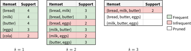
The candidate itemsets of each size \(k\), with their support. The frequent itemsets of size \(k - 1\) form the candidates of size \(k\), and the candidates with an infrequent subset are pruned without counting their support.
The transactions form a boolean matrix, with one row per transaction and one column per item, and the support of an itemset is the number of rows that hold all its items. The following function implements Apriori on this matrix, and returns the support of each frequent itemset:
import numpy as np

items = ['bread', 'milk', 'butter', 'eggs', 'cola']
T = np.array([[1, 1, 0, 0, 0],  # one transaction per row, one item per column
              [1, 0, 1, 1, 0],
              [0, 1, 1, 1, 1],
              [1, 1, 1, 1, 0],
              [1, 1, 1, 0, 1]], dtype=bool)

def apriori(T, min_support):
    L = {frozenset([i]): s for i, s in enumerate(T.sum(0)) if s >= min_support}
    frequent = dict(L)
    while L:
        C = {a | b for a in L for b in L if len(a | b) == len(a) + 1}  # join
        C = [X for X in C if all(X - {i} in L for i in X)]  # prune
        L = {X: T[:, list(X)].all(1).sum() for X in C}  # scan: the support of X
        L = {X: s for X, s in L.items() if s >= min_support}
        frequent.update(L)
    return frequent  # the support of each frequent itemset
Apriori scans the database once per itemset size, and the number of candidates grows very large when the minimum support is low.
ECLAT and FP-Growth
ECLAT (Equivalence Class Transformation) stores, for each item, the set of the transactions that hold it, its tidset. The support of an itemset is then the size of the intersection of the tidsets of its items, with no scan of the database. ECLAT searches the itemsets depth-first, extending each itemset with one item at a time, which is fast as long as the tidsets fit in memory. In the boolean matrix above, the tidset of an item is its column, and the intersection of two tidsets is the logical AND of their columns:
def eclat(T, min_support, prefix=(), tids=None):
    tids = np.ones(len(T), bool) if tids is None else tids  # the tidset of the prefix
    frequent = {}
    for i in range(prefix[-1] + 1 if prefix else 0, T.shape[1]):  # each later item
        t = tids & T[:, i]  # the intersection of the two tidsets
        if t.sum() >= min_support:
            frequent[frozenset(prefix + (i,))] = t.sum()
            frequent.update(eclat(T, min_support, prefix + (i,), t))  # depth-first
    return frequent
FP-growth (Frequent Pattern growth) generates no candidates at all. It scans the database twice: first, to count the support of each item; then, to insert the frequent items of each transaction, sorted by decreasing support, into a prefix tree, the FP-tree. Transactions that share a prefix share a path in the tree, and each node counts the transactions that pass through it, so the tree is a compressed copy of the database. Then, for each item, from the least frequent one, FP-growth collects the paths of the tree that end at that item (its conditional pattern base), builds a smaller FP-tree from them, and mines it recursively. The following picture illustrates the FP-tree of the transactions above, and the mining of eggs:
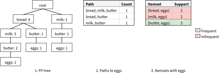
1. The FP-tree of the transactions, with the number of transactions that pass through each node. 2. The conditional pattern base of eggs: the paths from the root to each node of eggs. 3. The support of each item of these paths together with eggs: only {butter, eggs} is frequent.
The following function implements FP-growth, with the FP-tree as nested dictionaries. It takes the transactions as pairs of items and counts, the form of the conditional pattern bases that it mines recursively, e.g. fp_growth([(np.flatnonzero(t), 1) for t in T], 3):
def fp_growth(T, min_support, suffix=()):
    counts = {}
    for items, c in T:  # first scan: the support of each item
        for i in items:
            counts[i] = counts.get(i, 0) + c
    order = [i for i in counts if counts[i] >= min_support]  # the frequent items,
    order.sort(key=lambda i: -counts[i])  # by decreasing support
    tree = {}  # the FP-tree, as nested {item: [count, children]}
    for items, c in T:  # second scan: insert the frequent items of each transaction
        node = tree
        for i in sorted([i for i in items if i in order], key=order.index):
            entry = node.setdefault(i, [0, {}])
            entry[0] += c
            node = entry[1]
    frequent = {}
    for i in reversed(order):  # each item, from the least frequent one
        frequent[frozenset(suffix + (i,))] = counts[i]
        base = [(path, c) for path, j, c in nodes(tree) if j == i]  # its pattern base
        frequent.update(fp_growth(base, min_support, suffix + (i,)))
    return frequent

def nodes(tree, path=()):  # each node, with the items on its path from the root
    for i, (c, children) in tree.items():
        yield path, i, c
        yield from nodes(children, path + (i,))
In practice, FP-growth is usually faster than Apriori, as it scans the database only twice and generates no candidates, while ECLAT is fast on dense datasets whose tidsets fit in memory.
Outlier Detection
Anomaly detection (or outlier detection) finds the data points that differ much from the rest of the data, such as fraudulent transactions or failing machines. Some clustering methods already detect outliers: DBSCAN labels them as noise, and a Gaussian mixture gives them a low likelihood. The two methods of this section are dedicated to the task, and give each point an anomaly score.
Isolation Forest
An isolation forest is based on the observation that anomalies are few and different, so they are easier to isolate than normal points. An isolation tree splits the data recursively: each node picks a random feature and a random split value between the minimum and the maximum of that feature, until each point is alone in a leaf. An anomaly, far from the other points, is isolated after a few splits, close to the root, while a point in a dense region needs many:
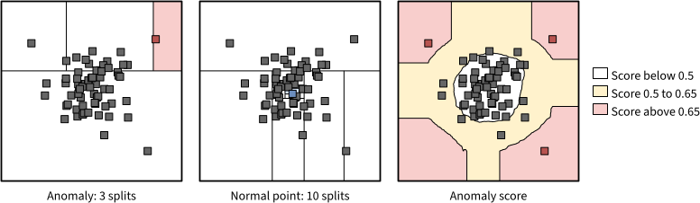
Points of a 2D Gaussian and 3 anomalies. Left and center: the random splits of an isolation tree, until an anomaly (red) or a normal point (blue) is alone in its cell. Right: the anomaly score of a forest of trees built on all the points. The splits are parallel to the axes, which gives the score map its cross shape.
The anomaly score of a point \(x\) is computed from its path length \(h(x)\), the number of splits from the root to its leaf, averaged over the trees of the forest:
\[s(x, m) = 2^{- \mathbb{E}[h(x)] / c(m)}\]where \(m\) is the number of points of each tree, and \(c(m) = 2 H(m-1) - 2(m-1)/m\) normalizes \(h(x)\). It is the average path length of an unsuccessful search in a binary search tree of \(m\) points, with the harmonic number \(H(i) \approx \ln(i) + 0.5772\). A score close to 1 marks an anomaly, and a score well below 0.5 a normal point.
Each tree is built on a small random subsample of the data, and its depth can be limited to about \(\log_2 m\), as only the short paths matter. Thus, an isolation forest computes no distances, its cost grows linearly with the number of points, and it scales to large datasets. The following functions implement it, with each tree as nested tuples, with the feature and the value of each split, and each leaf as its number of points:
def c(n):  # the average path length of an unsuccessful search in a BST of n points
    if n <= 2:
        return 1.0 if n == 2 else 0.0
    return 2 * (np.log(n - 1) + 0.5772) - 2 * (n - 1) / n

def isolation_tree(X, depth, rng):  # a node (f, s, left, right), or the leaf size
    if depth == 0 or len(X) <= 1:
        return len(X)
    f = rng.integers(X.shape[1])  # a random feature, and a random split value
    s = rng.uniform(X[:, f].min(), X[:, f].max())
    left = X[:, f] < s
    return (f, s, isolation_tree(X[left], depth - 1, rng),
            isolation_tree(X[~left], depth - 1, rng))

def path_length(x, node):  # h(x): the depth of x, plus c(n) in a leaf of n points
    if not isinstance(node, tuple):
        return c(node)
    f, s, left, right = node
    return 1 + path_length(x, left if x[f] < s else right)

def isolation_forest(X, trees=100, m=256, seed=0):
    rng = np.random.default_rng(seed)
    m = min(m, len(X))  # the number of points of each tree
    depth = int(np.ceil(np.log2(m)))  # the maximum depth of a tree
    forest = [isolation_tree(X[rng.choice(len(X), m, replace=False)], depth, rng)
              for _ in range(trees)]
    h = np.array([[path_length(x, tree) for tree in forest] for x in X])
    return 2 ** (-h.mean(1) / c(m))  # the anomaly score s(x, m)
Local Outlier Factor
The local outlier factor (LOF) compares the density around a point with the density around its neighbors. A point in a sparse region is not an outlier when its neighbors lie in a sparse region too, so LOF also finds outliers in data with clusters of different densities, where a single distance threshold fails. With the \(k\) nearest neighbors \(N_k(p)\) of a point \(p\), and the distance \(d_k(o)\) from a point \(o\) to its \(k\)-th nearest neighbor:
- the reachability distance of \(p\) from \(o\) is \(\text{reach}_k(p, o) = \max \{ d_k(o), d(p, o) \}\), i.e. the distance between them, but at least \(d_k(o)\), which smooths the distances within a dense region;
- the local reachability density of \(p\) is the inverse of its average reachability distance from its neighbors:
- the LOF of \(p\) is the average ratio between the densities of its neighbors and its own:
A LOF close to 1 means that the point is as dense as its neighbors, and a LOF much larger than 1 that it is an outlier. The following picture compares LOF with a global method, the distance to the \(k\)-th nearest neighbor:
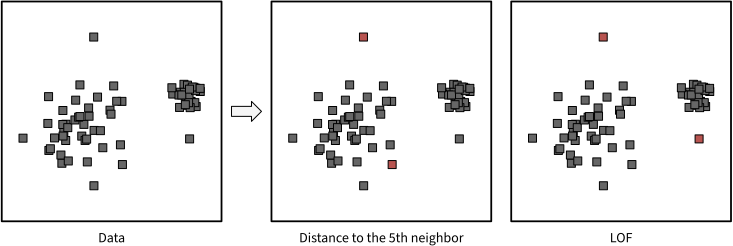
A sparse cluster, a dense cluster, a global outlier (top) and a local outlier under the dense cluster, with the two points of highest score of each method in red, for \(k = 5\). The distance to the 5th nearest neighbor flags the global outlier and a point of the sparse cluster, while LOF flags both outliers.
The following function computes the LOF of each point:
def lof(X, k):
    D = np.sqrt(((X[:, None] - X) ** 2).sum(2))
    np.fill_diagonal(D, np.inf)  # a point is not its own neighbor
    N = np.argsort(D, 1)[:, :k]  # the k nearest neighbors of each point
    rows = np.arange(len(X))[:, None]
    dk = D[rows[:, 0], N[:, -1]]  # the distance to the k-th nearest neighbor
    reach = np.maximum(dk[N], D[rows, N])  # reach_k(p, o), for each neighbor o of p
    lrd = 1 / reach.mean(1)
    return lrd[N].mean(1) / lrd
LOF needs the \(k\) nearest neighbors of each point, i.e. \(O(n^2)\) distances with a brute-force search. For the sake of comparison, an isolation forest is faster and scales to large datasets, while LOF finds the local outliers next to a dense cluster that a global method may miss.