Variational Autoencoders (VAEs) and Generative Adversarial Networks (GANs)
Variational Autoencoders (VAEs) and Generative Adversarial Networks (GANs) are two generative models based on neural networks, for distributions that no standard parametric family describes. The VAE builds on Variational Inference, which approximates an intractable posterior distribution by a simpler, parametric one.
Variational Autoencoder (VAE)
This section follows the papers Auto-Encoding Variational Bayes and An Introduction to Variational Autoencoders, by Diederik P. Kingma and Max Welling.
The papers introduce Variational Autoencoders, to perform efficient inference and learning in probabilistic models whose latent variables and parameters have intractable posterior distributions, on large datasets. The Stochastic Gradient Variational Bayes (SGVB) estimator of the variational lower bound (the ELBO, below) can be used for efficient approximation of posterior inference in almost any model with continuous latent variables, and, because it is differentiable, it can be optimized with stochastic gradient descent. The Auto-Encoding Variational Bayes (AEVB) algorithm uses the SGVB estimator to optimize a model that does efficient approximate posterior inference using simple sampling (from parametric distributions).
Autoencoders and variational autoencoders
An autoencoder (AE) is a neural network trained to reproduce its input: an encoder maps the input \(x\) to a code \(z\), usually of fewer dimensions, and a decoder maps the code back to a reconstruction \(\hat{x}\) of the input. The loss compares \(\hat{x}\) with \(x\), e.g. with the squared error, so that the code keeps the information needed to rebuild the input.
The VAE is a probabilistic autoencoder, where the probabilistic encoder \(q_\phi(z \mid x)\) (aka recognition model) and decoder \(p_\theta(x \mid z)\) (aka generative model) are represented as neural networks, with parameters \(\phi\) and \(\theta\). The decoder is a Gaussian or a Bernoulli distribution, whose parameters are computed from \(z\). Therefore, the VAE can be viewed as two coupled, independently parameterized models, trained together, where the encoder delivers to the decoder an approximation of its posterior over the latent variables. The AEVB algorithm finds the parameters of both, i.e. it performs approximate variational inference in the directed graphical model of the VAE.
The difference between Variational Autoencoders and regular Autoencoders (and other encoder-decoders, such as sequence-to-sequence models) is that:
- in regular AEs, the latent representation \(z\) is both the output of the encoder and the input of the decoder;
- in VAEs, the outputs of the encoder are the parameters of the distribution of \(z\) (e.g. the mean and variance in the case of a Gaussian distribution), and \(z\) is drawn from the distribution with those parameters and then passed to the decoder;
In practice, they can be visualized as follows, with the path of the AE at the top and the path of the VAE at the bottom of the dashed frame:
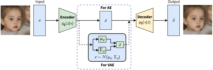
Adapted from: Variational Autoencoders, S. Yadav, Data Science Blog
The latent variable model
The VAE assumes that each datapoint \(x^{(i)}\) of a dataset of i.i.d. samples is generated by a random process of two steps, which involves an unobserved continuous random variable \(z\):
- a value \(z^{(i)}\) is generated from some prior distribution \(p_{\theta^*}(z)\); and
- a value \(x^{(i)}\) is generated from the likelihood distribution \(p_{\theta^*}(x \mid z)\).
Think of \(z\) as the hidden factors of a datapoint: for an image of a handwritten digit, which digit it is, its slant and the thickness of its stroke. The likelihood then draws the pixels of the image from these factors.
The assumptions are that both the prior and likelihood functions are parametric differentiable distributions, and that the true parameters \(\theta^*\) and the latent values \(z^{(i)}\) are unknown. There is also an assumption of intractability, as in:
- the integral of the evidence or marginal likelihood \(p_\theta(x) = \int p_\theta(z) \, p_\theta(x \mid z) \, dz\) is intractable, so it can be neither evaluated nor differentiated;
- the true posterior density \(p_\theta(z \mid x) = p_\theta(x \mid z) \, p_\theta(z) / p_\theta(x)\) is intractable, as it divides by this integral, so the expectation maximization algorithm cannot be used; and
- the integrals required by any mean-field approximation algorithm are also intractable.
This is the level of intractability common to DNNs with nonlinear hidden layers.
The encoder and amortized inference
The paper proposes an efficient approximation of the Maximum Likelihood (MLE) or Maximum a Posteriori (MAP) estimation of the parameters \(\theta\), of the posterior inference of the latent variable \(z\), and of the marginal inference of the variable \(x\). Similarly to other variational inference methods, the intractable true posterior \(p_{\theta}(z \mid x)\) is approximated by \(q_\phi(z \mid x)\) (the encoder), whose parameters \(\phi\) are not computed by a closed-form expectation but learned as the weights of the encoder network instead. Given a datapoint \(x\), the encoder produces a distribution over the possible values of the code \(z\) from which the datapoint \(x\) could have been generated.
The VAE of the paper takes the prior as the centered isotropic Gaussian \(p(z) = \mathcal{N}(0, I)\), which has no parameters, and the encoder as a Gaussian with a diagonal covariance, \(q_\phi(z \mid x) = \mathcal{N}(\mu, \operatorname{diag}(\sigma^2))\). The mean \(\mu\) and the standard deviation \(\sigma\), two vectors of the size of \(z\), are the outputs of the encoder network for the input \(x\) (\(\mu_z\) and \(\Sigma_z = \operatorname{diag}(\sigma^2)\) in the picture above).
One advantage of the VAE framework, relative to ordinary Variational Inference, is that the encoder is now a stochastic function of the input variables. In VI, each data-case has a separate variational distribution, which is inefficient for large datasets: the number of variational parameters grows with the dataset, and a new datapoint needs an optimization of its own. The encoder uses one set of parameters \(\phi\) for all datapoints, and computes the distribution of a new datapoint with one forward pass, which is called amortized inference.
The loss function: the ELBO
The VAE maximizes the evidence lower bound (ELBO) of each datapoint, so its loss function is the negative of the ELBO. The ELBO is an expectation over the distribution of the encoder, which splits into the sum of two terms (Eq. 2 and 3 in the AEVB paper):
\[\begin{align*} \text{ELBO}(\theta, \phi; x) & = \mathbb{E}_{q_\phi(z \mid x)} \left[ \log p_\theta(x, z) - \log q_\phi(z \mid x) \right] \\ & = \mathbb{E}_{q_\phi(z \mid x)} \left[ \log p_\theta(x \mid z) \right] - \text{KL} \big( q_\phi(z \mid x) \parallel p(z) \big) \end{align*}\]The first term is the expected log-likelihood of the datapoint, and its negative is the reconstruction loss (the paper calls this term an expected negative reconstruction error). The expectation is taken with respect to the encoder’s distribution over the representations, encouraging the VAE to generate valid datapoints. This loss compares the model output with the model input. It can be any of the losses used in regular autoencoders, such as the L2 loss (for a Gaussian decoder with a fixed variance), the cross-entropy (for a Bernoulli decoder), etc.
The second term is the Kullback-Leibler divergence (KL) between the encoder’s distribution \(q_{\phi}(z \mid x)\) and the prior \(p(z) = \mathcal{N}(0, I)\), a zero-mean, unit-variance Gaussian. This divergence acts as a regularizer, as the paper calls it: it penalizes the VAE if the encoder outputs representations \(z\) that are different from those of a standard normal distribution. Without it, the encoder could give each datapoint a representation in a different region of the latent space.
With a Gaussian encoder and a Gaussian prior, this KL divergence has a closed form (Appendix B of the paper), so it needs no sampling. For a latent space of \(J\) dimensions, it is computed as:
\[\text{KL} \big( q_\phi(z \mid x) \parallel p(z) \big) = \frac{1}{2} \sum_{j=1}^{J} \left( \mu_j^2 + \sigma_j^2 - 1 - \log \sigma_j^2 \right)\]where \(\mu_j\) and \(\sigma_j\) are the mean and the standard deviation of the \(j\)-th dimension of \(z\). The penalty is zero only when \(\mu_j = 0\) and \(\sigma_j = 1\), i.e. when the encoder outputs the prior: the term \(\mu_j^2\) pulls the means toward 0, and the terms \(\sigma_j^2 - \log \sigma_j^2\) keep the standard deviations close to 1. The reconstruction term pulls the other way, toward precise codes (a small \(\sigma_j\)) that tell the datapoints apart, and the ELBO balances the two.
The ELBO is a lower bound of the log-likelihood, because the log-likelihood of a datapoint is the ELBO plus the KL divergence of the encoder from the true posterior, which is never negative (Eq. 1 in the paper):
\[\log p_\theta(x) = \text{ELBO}(\theta, \phi; x) + \text{KL} \big( q_\phi(z \mid x) \parallel p_\theta(z \mid x) \big) \ge \text{ELBO}(\theta, \phi; x)\]Therefore, maximizing the ELBO with respect to \(\theta\) and \(\phi\) does two things at once (section 2.2.1 of the Introduction to Variational Autoencoders): it approximately maximizes the likelihood \(p_\theta(x)\), so the decoder becomes a better generative model, and it minimizes the KL divergence of the encoder from the true posterior, so the encoder becomes a better approximation of it.
The reparameterization trick
The loss is minimized with stochastic gradient descent, which needs the gradient of the ELBO with respect to the parameters \(\phi\) of the encoder. The authors noticed that the sampling induces noise in this gradient (or, put differently, that \(z\) is randomly generated and cannot be backpropagated): the first term of the ELBO is an expectation over \(q_\phi(z \mid x)\), a distribution that depends on \(\phi\) itself. The usual Monte Carlo estimator of such a gradient, the score function estimator (also called REINFORCE), is computed as:
\[\nabla_\phi \mathbb{E}_{q_\phi(z \mid x)} \left[ f(z) \right] = \mathbb{E}_{q_\phi(z \mid x)} \left[ f(z) \, \nabla_\phi \log q_\phi(z \mid x) \right]\]where \(f(z) = \log p_\theta(x \mid z)\) is the objective. It uses only the value of \(f\), not its gradient, and it has a very high variance, which makes it impractical (section 2.2 of the paper). To counteract that, the authors propose the reparameterization trick.
The reparameterization trick moves the randomness of the sampling into an auxiliary noise variable, through a deterministic transformation. Instead of sampling \(z \sim \mathcal{N}(\mu, \sigma^2)\), \(z\) is rewritten as \(z = \mu + \sigma \cdot \epsilon\), where \(\epsilon\) follows the standard Gaussian, i.e. \(\epsilon \sim \mathcal{N}(0, 1)\). For a vector \(z\), the product is element-wise, \(z = \mu + \sigma \odot \epsilon\), with \(\epsilon \sim \mathcal{N}(0, I)\).
Why does this work?
- The randomness is now isolated in \(\epsilon\), which does not depend on the model parameters.
- The computation of \(z\) becomes a differentiable function of \(\mu\) and \(\sigma\) (the outputs of the encoder), allowing gradients to flow through \(\mu\) and \(\sigma\) during backpropagation, because the transformation \(z = \mu + \sigma \cdot \epsilon\) is fully differentiable with respect to these parameters.
In practice, the derivatives are \(\partial z / \partial \mu = 1\) and \(\partial z / \partial \sigma = \epsilon\): the gradient of the objective reaches the encoder through \(z\) by the chain rule, as through any other layer, and its estimate is much less noisy than that of the score function estimator.
The following picture illustrates the computation graph of the objective before and after the reparameterization:
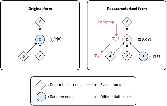
Illustration of the reparameterization trick. The variational parameters ϕ affect the objective f through the random variable z ~ qϕ(z|x). Optimizing the objective with SGD requires the gradients ∇ϕf. In the original form (left), f cannot be differentiated with respect to ϕ, because gradients cannot be backpropagated through the random variable z. The reparameterized form (right) externalizes the randomness of z by writing it as a deterministic and differentiable function of ϕ, x and a new random variable ε. Gradients then flow through z, and ∇ϕf can be computed. Adapted from: An Introduction to Variational Autoencoders
Putting the pieces together gives the SGVB estimator of the ELBO of a datapoint (Eq. 10 in the paper), with one sample of the noise per datapoint, as in the experiments of the paper:
\[\text{ELBO}(\theta, \phi; x) \approx \log p_\theta(x \mid z) - \frac{1}{2} \sum_{j=1}^{J} \left( \mu_j^2 + \sigma_j^2 - 1 - \log \sigma_j^2 \right)\]where \(z = \mu + \sigma \odot \epsilon\) is computed from one sample \(\epsilon \sim \mathcal{N}(0, I)\). In practice, a training step passes each datapoint of a mini-batch through the encoder to get \(\mu\) and \(\sigma\), samples \(\epsilon\) and computes \(z\). Then, it passes \(z\) through the decoder to get the reconstruction term, adds the closed-form KL, and backpropagates the negative of the result, the loss, through both networks.
Generating new data
Once the VAE is trained, the encoder is not needed to generate data: a sample of the prior, \(z \sim \mathcal{N}(0, I)\), passes through the decoder, and the mean of \(p_\theta(x \mid z)\) (e.g. the intensity of each pixel of an image) is a new datapoint. This works because the KL term kept the codes of the training data close to the prior, so that a sample of the prior falls where the decoder was trained. With a two-dimensional \(z\), the paper decodes a grid of codes into a map of the digits that the decoder generates across the latent space (Figure 4 of the paper). The encoder remains useful to map a datapoint to its latent representation, e.g. to compare datapoints.
Generative Adversarial Network (GAN)
This section follows the paper Generative Adversarial Networks, by Ian Goodfellow and colleagues (NIPS 2014).
The paper introduces a new generative model composed of two models trained simultaneously:
- a generative model G that captures the data distribution; and
- a discriminative model D that estimates the probability that a sample came from the training data rather than G;
The training procedure for G is to maximize the probability of D making a mistake. This framework corresponds to a minimax two-player game. The name adversarial comes from the fact that the generative model faces the discriminative model, which learns whether a sample is from the model distribution or from the data distribution. Quoting the authors:
“The generative model can be thought of as analogous to a team of counterfeiters, trying to produce fake currency and use it without detection, while the discriminative model is analogous to the police, trying to detect the counterfeit currency. Competition in this game drives both teams to improve their methods until the counterfeits are indistiguishable from the genuine articles.”
Compared with the VAE, a GAN generates sharper samples, but it has no encoder and no bound on the likelihood of the data, and it is harder to train.
Mathematical setup
The goal of the generative model is to generate samples by passing random noise \(z\) through a multilayer perceptron.
- The generator \(G(z; \theta_g)\) is a multilayer perceptron with parameters \(\theta_g\).
- \(p_z(z)\) is the prior on the input noise variables.
- The generator \(G\) implicitly defines a probability distribution \(p_g\) as the distribution of the samples \(G(z)\) obtained when \(z \sim p_z\);
- The goal of the generator is to make \(p_g\) close to the distribution of the data \(p_\text{data}\), to fake it “well enough” and trick the discriminator;
The discriminative model is also a multilayer perceptron.
- The discriminator \(D(x; \theta_d)\) takes the input \(x\) and, based on its DNN parameters \(\theta_d\), outputs a single scalar representing the probability that \(x\) came from the data rather than \(p_g\);
The overall structure of the generator and discriminator training can be pictured as:
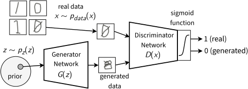
Adapted from: Benjamin Striner, lecture notes on GANs, CMU 11-785 Introduction to Deep Learning
The minimax loss
The discriminator \(D\) is trained to best guess the source of the data, i.e. to maximize the probability of assigning the correct label to both the training examples and the samples from \(G\).
The generator \(G\) is simultaneously trained to minimize \(\log(1-D(G(z)))\), i.e. to be able to fake the data well enough. In practice, \(D\) and \(G\) are playing a two-player minimax game with value function \(V(D, G)\):
\[\min_G \max_D V(D, G) = \mathbb{E}_{\boldsymbol{x} \sim p_{\text{data}}(\boldsymbol{x})} [\log D(\boldsymbol{x})] + \mathbb{E}_{\boldsymbol{z} \sim p_{\boldsymbol{z}}(\boldsymbol{z})} [\log (1 - D(G(\boldsymbol{z})))].\]The loss function is a sum of two penalization terms:
- in the first term, the discriminator is optimized such that, in the long run, all real inputs (drawn from the data, i.e. \(x \sim p_\text{data}\)) are expected to be classified as correctly as possible;
- in the second term, the discriminator and the generator are optimized with opposite goals on all fake inputs (generated by the generator from \(z \sim p_z\)): the discriminator maximizes this term, to classify fake inputs as fake, and the generator minimizes it, so that the discriminator classifies fake inputs as real;
Finally, notice there is a \(\log\) term added to both expected value terms. This is because the objective function is the product of multiple probabilities (of \(D\) assigning the correct label to each input), in this case \(D(x) * (1-D(G(z)))\). Adding the \(\log\) makes the optimization return the same optima (as \(\log\) is monotonic), while making it faster and more numerically stable. The expectation term is also added to the loss because the goal is to minimize the loss that is expected after several samples (law of large numbers). Thus:
\[\mathbb{E} \left[ \log(D(x) * (1-D(G(z)))) \right] = \mathbb{E} \left[ \log(D(x)) \right] + \mathbb{E} \left[ \log(1-D(G(z))) \right]\]In other words, \(V(D, G)\) is the negative of the binary cross-entropy of \(D\), the standard loss of a binary classifier, with the label 1 for real inputs and 0 for generated ones: the discriminator maximizes \(V\) by minimizing its classification loss, and the generator minimizes \(V\) by maximizing it.
In section 4 (theoretical results), the authors show that, given enough capacity for the discriminator and the generator, the minimax game recovers the data-generating distribution. For a fixed generator, the optimal discriminator is given by (Proposition 1 in the paper):
\[D^*_G(x) = \frac{p_\text{data}(x)}{p_\text{data}(x) + p_g(x)}\]i.e. the probability that a sample at \(x\) comes from the data rather than from the generator, when both are drawn equally often. Where \(p_g(x) = p_\text{data}(x)\), it outputs \(1/2\): it cannot tell the two apart.
With the optimal discriminator, the value function becomes the criterion that the generator minimizes, \(C(G) = \max_D V(D, G)\), which is computed as (in the proof of Theorem 1 of the paper):
\[C(G) = -\log 4 + 2 \cdot \text{JSD}(p_\text{data} \parallel p_g)\]where JSD is the Jensen-Shannon divergence, the mean of the KL divergences of \(p_\text{data}\) and \(p_g\) from their average \((p_\text{data} + p_g) / 2\). Unlike the KL divergence, it is symmetric, and it ranges from 0, when the two distributions are equal, to \(\log 2\), when they do not overlap. Therefore, this minimax game has a global optimum, \(C(G) = -\log 4\), reached only when \(p_g = p_\text{data}\).
However, the proof that the training algorithm converges to this optimum (Proposition 2 in the paper) assumes that \(D\) reaches its optimum given \(G\) at every step, and that \(p_g\) itself is updated. In practice, the algorithm updates the parameters \(\theta_g\) of a multilayer perceptron, which introduces multiple critical points in the parameter space, and the authors use it despite its lack of theoretical guarantees.
Training algorithm
The training algorithm is the following:
\[\begin{array}{l} \hline \textbf{Algorithm 1} \text{ Minibatch stochastic gradient descent training of generative} \\ \text{adversarial nets. The number of steps to apply to the discriminator, } k \text{, is a} \\ \text{hyperparameter. We used } k = 1 \text{, the least expensive option, in our experiments.} \\ \hline \quad \textbf{for} \text{ number of training iterations } \textbf{do} \\ \qquad \textbf{for}\ k \text{ steps } \textbf{do} \\ \qquad\quad \bullet \text{ Sample minibatch of } m \text{ noise samples } \{\boldsymbol{z}^{(1)}, \ldots, \boldsymbol{z}^{(m)}\} \text{ from noise prior } p_{\boldsymbol{z}}(\boldsymbol{z}). \\ \qquad\quad \bullet \text{ Sample minibatch of } m \text{ examples } \{\boldsymbol{x}^{(1)}, \ldots, \boldsymbol{x}^{(m)}\} \text{ from data generating distribution} \\ \qquad\quad p_{\text{data}}(\boldsymbol{x}). \\ \qquad\quad \bullet \text{ Update the discriminator by ascending its stochastic gradient:} \\ \hspace{9em} \displaystyle \nabla_{\theta_d} \frac{1}{m} \sum_{i=1}^m \left[ \log D\left(\boldsymbol{x}^{(i)}\right) + \log\left(1 - D\left(G\left(\boldsymbol{z}^{(i)}\right)\right)\right) \right]. \\ \qquad \textbf{end for} \\ \qquad \bullet \text{ Sample minibatch of } m \text{ noise samples } \{\boldsymbol{z}^{(1)}, \ldots, \boldsymbol{z}^{(m)}\} \text{ from noise prior } p_{\boldsymbol{z}}(\boldsymbol{z}). \\ \qquad \bullet \text{ Update the generator by descending its stochastic gradient:} \\ \hspace{12.8em} \displaystyle \nabla_{\theta_g} \frac{1}{m} \sum_{i=1}^m \log\left(1 - D\left(G\left(\boldsymbol{z}^{(i)}\right)\right)\right). \\ \quad \textbf{end for} \\ \text{The gradient-based updates can use any standard gradient-based learning rule.} \\ \text{We used momentum in our experiments.} \\ \hline \end{array}\]Challenge: different convergence speeds of the generator and the discriminator
Optimizing \(D\) to completion before each step of \(G\) is “computationally prohibitive, and on finite datasets would result in overfitting”. Instead, training alternates between \(k\) steps of optimizing \(D\) and one step of optimizing \(G\) (the authors use \(k=1\)). This keeps \(D\) near its optimal solution, as long as \(G\) changes slowly enough.
Challenge: saturation of the generator loss
The loss equation may not provide sufficient gradient for \(G\) to learn well. Early in learning, when \(G\) is poor, \(D\) can reject samples with high confidence because they are clearly different from the training data. In this case, \(\log(1 − D(G(z)))\) saturates.
Saturation means that \(D(G(z))\) is close to 0, where this term is flat. The output of \(D\) is the sigmoid of a logit \(a\), \(D = \operatorname{sigmoid}(a)\), and the derivative of \(\log(1 - \operatorname{sigmoid}(a))\) with respect to \(a\) is \(-\operatorname{sigmoid}(a)\), close to 0. In practice, this means that this term of the loss function will not provide any signal (gradients) for the update of the generator, making it useless: when the discriminator performs significantly better than the generator, the updates to the generator are either inaccurate or disappear.
This leads to two main problems:
- mathematically, the update of the parameters is zero or very small, so progress through the loss landscape is very slow;
- computationally, arithmetic operations over very small values lead to incorrect (or “always zero”) results due to insufficient floating-point precision in the processor (typically 16 or 32 bits);
The workaround suggested by the authors is to change the algorithm for training the generator: instead of minimizing \(\log(1 - D(G(z)))\), they maximize \(\log D(G(z))\), known as the non-saturating loss of the generator. This keeps the same fixed point of the dynamics of \(G\) and \(D\), while the optimization landscape “provides much stronger gradients early in learning”: the derivative of \(\log \operatorname{sigmoid}(a)\) with respect to \(a\) is \(1 - \operatorname{sigmoid}(a)\), close to 1. The pseudocode above shows the original update, which minimizes \(\log(1 - D(G(z)))\).
Challenge: mode collapse
The original publication mentions this challenge only briefly, as “the Helvetica scenario” in which \(G\) collapses too many values of \(z\) to the same value of \(x\). In a regular scenario, GANs are expected to generate a range of outputs, or ideally, a new random valid output for every random input to the generator. Instead, it may happen that sometimes the output is monotonous, i.e. a range of very similar outputs.
This phenomenon is called mode collapse and is detailed in this paper as: “This undesirable event occurs when the model can only fit a few modes of the data distribution, while ignoring the majority of them”. Proposed solutions include a different loss function (the Wasserstein loss) and Unrolled GANs, which incorporate the current and future discriminator’s classifications in the loss function, so that the generator cannot over-optimize for a single discriminator.