Variational Inference (ELBO, CAVI) and Gaussian Mixture Models
The previous Bayesian Linear Regression post showed that the goal of Bayesian inference is to compute the posterior, the distribution of the unknown variables (there, the weights of a linear regression) given the observed data. Recall the formulation of the posterior of the latent variables \(z\) given the observations \(x\), for a model with parameters \(\theta\), derived from the Bayes rule, with and without the normalization term:
\[p_\theta(z \mid x) = \frac{p_\theta(z) \, p_\theta(x \mid z)}{p_\theta(x)} \propto p_\theta(z) \, p_\theta(x \mid z)\]read as the posterior is proportional to the prior times the likelihood. The same post also showed that the Bayes rule derives from the definition of conditional probability \(p_\theta(z \mid x)\) expressed as:
\[p_\theta(z \mid x) = \frac{p_\theta(x, z)}{p_\theta(x)}\]where the denominator is the marginal density of the observations \(x\), also referred to as the evidence, which is computed by marginalizing out the latent variables \(z\) from the joint distribution:
\[p_\theta(x) = \int p_\theta(x, z) \, dz\]For many models, this evidence integral has no closed-form solution or requires exponential time to compute. The posterior is then intractable, and approximate inference methods are needed, such as Markov Chain Monte Carlo (MCMC) or variational inference.
Variational Inference
The idea behind Variational Inference (VI) methods is to approximate the intractable posterior \(p_\theta(z \mid x)\) by a simpler, parametric distribution \(q_\phi(z)\), with variational parameters \(\phi\). Inference thus becomes an optimization problem: instead of sampling from the posterior, as MCMC does, VI searches for the variational parameters \(\phi\) that bring \(q_\phi(z)\) closest to the posterior, while the model parameters \(\theta\) stay fixed. The closeness of the two distributions is measured by the Kullback–Leibler (KL) divergence of \(q_\phi(z)\) from the posterior, defined as:
\[\text{KL}(q_\phi(z) \parallel p_\theta(z \mid x)) = \int q_\phi(z) \log \frac{q_\phi(z)}{p_\theta(z \mid x)} \, dz = \mathbb{E}_{q_\phi} \left[ \log \frac{q_\phi(z)}{p_\theta(z \mid x)} \right] \label{eq_KLdiv}\]Note that the KL divergence is a dissimilarity function and not a metric, as it is not symmetric.
The order of the two distributions matters. Eq. \ref{eq_KLdiv}, written \(\text{KL}(q \parallel p)\) for short, is called the reverse KL divergence: it is an expectation over \(q\), which is chosen simple enough for this expectation to be computed, and the posterior only appears inside its logarithm. The forward KL divergence \(\text{KL}(p \parallel q)\) would instead be an expectation over the posterior \(p_\theta(z \mid x)\), the very distribution that is unknown.
Looking at eq. \ref{eq_KLdiv}, there is an issue: it includes the true posterior \(p_\theta(z \mid x)\), which is exactly the distribution that is not known. So it cannot be minimized directly, but it is possible to maximize a function that is equal to its negative (up to a constant), known as the Evidence Lower Bound.
Evidence Lower Bound (ELBO)
The KL divergence can be rewritten as:
\[\begin{align*} \text{KL}(q_\phi(z) \parallel p_\theta(z \mid x)) & = \int q_\phi(z) \log \frac{q_\phi(z)}{p_\theta(z \mid x)} \, dz \\ & = \int q_\phi(z) \log \frac{q_\phi(z) \, p_\theta(x)}{p_\theta(x, z)} \, dz \\ & \qquad \text{(definition of conditional probability)} \\ & = \int q_\phi(z) \left( \log p_\theta(x) + \log \frac{q_\phi(z)}{p_\theta(x, z)} \right) dz \\ & \qquad \text{(expanding the log)} \\ & = \log p_\theta(x) \int q_\phi(z) \, dz + \int q_\phi(z) \log \frac{q_\phi(z)}{p_\theta(x, z)} \, dz \\ & \qquad \text{(splitting the integral)} \\ & = \log p_\theta(x) - \int q_\phi(z) \log \frac{p_\theta(x, z)}{q_\phi(z)} \, dz \\ & \qquad \text{(negating the log; } q_\phi \text{ is a distribution, so } \textstyle \int q_\phi(z) \, dz = 1 \text{)} \\ & = \log p_\theta(x) - \text{ELBO}(\phi) \end{align*}\]Thus, the KL divergence, which could not be minimized, is replaced by an expression that can be optimized: minimizing the KL divergence is equivalent to maximizing the ELBO. Looking at the right-hand side of the expression:
- The goal is to minimize the KL divergence over \(\phi\), so the term \(\log p_\theta(x)\) can be ignored as it does not depend on \(\phi\);
- All terms inside \(\text{ELBO}(\phi)\) are known, as \(p_\theta(x, z)\) is the prior times the likelihood, \(p_\theta(x, z) = p_\theta(z) \, p_\theta(x \mid z)\), which are the inputs of the problem;
- The KL divergence cannot be negative, by Jensen’s inequality. Thus \(\log p_\theta(x) \ge \text{ELBO}(\phi)\), i.e. the ELBO is never larger than the log evidence \(\log p_\theta(x)\), and this explains the name Evidence Lower Bound.
The ELBO is usually written in terms of two expectations:
\[\begin{align} \text{ELBO}(\phi) & = \int q_\phi(z) \log \frac{p_\theta(x, z)}{q_\phi(z)} \, dz \\ & = \int q_\phi(z) \log p_\theta(x, z) \, dz - \int q_\phi(z) \log q_\phi(z) \, dz \\ & = \mathbb{E}_{q_\phi} [\log p_\theta(x, z)] - \mathbb{E}_{q_\phi} [\log q_\phi(z)] \label{eq_elbo} \end{align}\]The second term, \(-\mathbb{E}_{q_\phi}[\log q_\phi(z)]\), is the entropy of \(q_\phi\), a measure of how spread out it is. So the ELBO rewards a \(q_\phi\) that places its mass where the joint \(p_\theta(x, z)\) is high, and its entropy term keeps \(q_\phi\) spread out, rather than collapsed on the single most likely value of \(z\).
There are two common options to solve the previous optimization problem: coordinate ascent variational inference (CAVI), which optimizes the approximation of one latent variable at a time (slow, and requires deriving the formulation of the updates by hand), or stochastic optimization, as in Stochastic Variational Inference (faster on large datasets). Both optimize over a family of distributions simple enough for the expectations of the ELBO to be computed, such as the mean-field family of the next section.
Mean-field approximation
So far, \(q_\phi(z)\) was one distribution over all latent variables; now it is restricted to a family that makes the optimization tractable. One way to do so is to approximate the posterior probability using a simpler model, for example by assuming that a set of latent variables is independent of the other variables. Or full independence can be enforced among all latent variables given \(x\). This assumption is known as the mean-field approximation.
This method originates from mean-field theory. From Wikipedia:
“Mean-field theory […] studies the behavior of high-dimensional random (stochastic) models by studying a simpler model that approximates the original by averaging over degrees of freedom. […] The effect of all the other individuals on any given individual is approximated by a single averaged effect, thus reducing a many-body problem to a one-body problem.”
Note that, because the latent variables are assumed to be independent, the mean-field family usually does not contain the true posterior: in the Gaussian mixture model below, for example, the cluster assignments of the points depend on each other and on the cluster means, given the data.
Under this assumption, the variational distribution over the latent variables \(z = (z_1, ..., z_J)\) factorizes as:
\[q_\phi(z) = \prod_{j=1}^{J} q_j(z_j) \label{eq_posterior_mf}\]where each latent variable \(z_j\) is governed by its own variational factor, the density \(q_j(z_j)\), with its own variational parameters. Note that the variational family does not depend on the input data \(x\), which does not show up in the equation: it is the ELBO that connects \(q_\phi\) to the data and the model.
The latent variables can also be partitioned into \(R\) groups \(z_{G_1}, ..., z_{G_R}\), with one factor per group:
\[q_\phi(z) = \prod_{j=1}^{R} q_j(z_{G_j})\]This setup is often called generalized mean field, as opposed to the naive mean field of eq. \ref{eq_posterior_mf}. For the formulation to be complete, the parametric form of the individual variational factors would have to be specified. In principle, each can take on any parametric distribution appropriate to the corresponding random variable (e.g. a combination of Gaussian and Categorical distributions).
Coordinate Ascent Variational Inference
The main objective is to optimize the ELBO in mean-field variational inference, i.e. to choose the variational factors that maximize the ELBO (eq. \ref{eq_elbo}). A common approach is to use the coordinate ascent method, optimizing one variational factor \(q_j(z_j)\) at a time while holding the others fixed. The derivation below follows the lecture notes Variational Inference: Mean Field Approximation of the CMU course Probabilistic Graphical Models (10-708).
First, the probability chain rule factorizes the joint distribution of the observations and the latent variables as:
\[%source: assets: 10708-scribe-lecture13.pdf p_\theta(x, z) = p_\theta(x) \prod_{l=1}^{J} p_\theta(z_l \mid z_{1:(l-1)}, x)\]and the negative entropy, \(\mathbb{E}_{q_\phi} [\log q_\phi(z)]\), can be decomposed using the mean-field factorization (eq. \ref{eq_posterior_mf}) as:
\[\mathbb{E}_{q_\phi} [\log q_\phi(z)] = \sum_{l=1}^{J} \mathbb{E}_{q_l} [\log q_l(z_l)]\]Inserting the two previous decompositions into the ELBO (eq. \ref{eq_elbo}), it can now be expressed for the mean-field family as:
\[%source: assets: 10708-scribe-lecture13.pdf \begin{align*} \text{ELBO}(\phi) & = \mathbb{E}_{q_\phi} [\log p_\theta(x, z)] - \mathbb{E}_{q_\phi} [\log q_\phi(z)] \\ & = \mathbb{E}_{q_\phi} \left[ \log \left( p_\theta(x) \prod_{l=1}^{J} p_\theta(z_l \mid z_{1:(l-1)}, x) \right) \right] - \sum_{l=1}^{J} \mathbb{E}_{q_l} [\log q_l(z_l)] \\ & = \log p_\theta(x) + \sum_{l=1}^{J} \mathbb{E}_{q_\phi} \left[ \log p_\theta(z_l \mid z_{1:(l-1)}, x) \right] - \sum_{l=1}^{J} \mathbb{E}_{q_l} [\log q_l(z_l)] \end{align*}\]The update of \(q_j\), with the other factors fixed, uses the complete conditional of \(z_j\), its distribution given all the other latent variables and the observations:
\[p_\theta(z_j \mid z_{-j}, x) = p_\theta(z_j \mid z_1, ..., z_{j-1}, z_{j+1}, ..., z_J, x)\]where \(z_{-j}\) denotes all the latent variables except \(z_j\). The goal is now to compute \(\arg\max_{q_j} \text{ELBO}\). The order of the latent variables in the chain rule is arbitrary, so \(z_j\) can be placed last, and then only the term \(p_\theta(z_j \mid z_{-j}, x)\) of the product depends on \(z_j\):
\[\begin{align*} & \arg\max_{q_j} \text{ELBO} \\ ={} & \arg\max_{q_j} \left( \log p_\theta(x) + \sum_{l=1}^{J} \mathbb{E}_{q_\phi} \left[ \log p_\theta(z_l \mid z_{1:(l-1)}, x) \right] - \sum_{l=1}^{J} \mathbb{E}_{q_l} [\log q_l(z_l)] \right) \\ ={} & \arg\max_{q_j} \left( \mathbb{E}_{q_\phi} \left[ \log p_\theta(z_j \mid z_{-j}, x) \right] - \mathbb{E}_{q_j} [\log q_j(z_j)] \right) \\ & \qquad \text{(removing the terms that do not depend on } q_j \text{)} \\ ={} & \arg\max_{q_j} \left( \int q_j(z_j) \, \mathbb{E}_{q_{-j}} \left[ \log p_\theta(z_j \mid z_{-j}, x) \right] dz_j - \int q_j(z_j) \log q_j(z_j) \, dz_j \right) \\ & \qquad \text{(definition of the expected value)} \end{align*}\]where \(\mathbb{E}_{q_{-j}}\) is the expectation over all the factors except \(q_j\). To find this argmax, a Lagrange multiplier \(\lambda\) is added for the constraint \(\int q_j(z_j) \, dz_j = 1\), as \(q_j\) is a distribution, and the derivative with respect to \(q_j(z_j)\) is set to zero:
\[\mathbb{E}_{q_{-j}} \left[ \log p_\theta(z_j \mid z_{-j}, x) \right] - \log q_j(z_j) - 1 + \lambda = 0\]Solving for \(q_j(z_j)\) gives \(q_j(z_j) = e^{\lambda - 1} \exp \left( \mathbb{E}_{q_{-j}} [\log p_\theta(z_j \mid z_{-j}, x)] \right)\), in which the factor \(e^{\lambda - 1}\) is the normalization constant that makes \(q_j(z_j)\) integrate to one. This leads to the final coordinate ascent update:
\[\begin{align} q_j^\star(z_j) & \propto \exp \left( \mathbb{E}_{q_{-j}} [\log p_\theta(z_j \mid z_{-j}, x)] \right) \\ & \propto \exp \left( \mathbb{E}_{q_{-j}} [\log p_\theta(x, z)] \right) \label{eq_CAVI} \\ & \qquad \text{(} p_\theta(x, z_{-j}) \text{ does not depend on } z_j \text{)} \end{align}\]This update provides the template of the computation, but not the final form (i.e. the distribution family) of the optimal \(q_j\): the form follows from the expectation in eq. \ref{eq_CAVI}, once it is computed for a specific model, and it determines the complexity or easiness of the coordinate update \(q_j^\star(z_j)\). When the complete conditional \(p_\theta(z_j \mid z_{-j}, x)\) is in the exponential family, the optimal factor is in the same family, and the update reduces to a closed-form formula for its variational parameters (section 4.1 of Variational Inference: A Review for Statisticians). The Gaussian mixture model of the next section is such a model.
Gaussian Mixture Models
This section follows sections 2.1 and 3 of the paper Variational Inference: A Review for Statisticians.
A Gaussian mixture model is a probabilistic model that assumes all the data points are generated from a mixture of a finite number of Gaussian distributions with unknown parameters. The problem at hand is to fit a set of Gaussian density functions to the input dataset.
Take a mixture of \(K\) univariate Gaussian distributions with means \(\mu = (\mu_1, ..., \mu_K)\), drawn from a common Gaussian prior \(\mathcal{N}(0, \sigma^2)\). The latent variables are the means \(\mu\) and the cluster assignments \(c = (c_1, ..., c_n)\) of the \(n\) observations \(x = (x_1, ..., x_n)\), i.e. \(z = \{\mu, c\}\). The prior variance \(\sigma^2\) is a hyperparameter: it plays the role of the model parameters \(\theta\), and it is omitted from the notation below.
Each assignment \(c_i\) is an indicator vector of size \(K\), i.e. all zeros except for a one at the index of its cluster. Each observation \(x_i\) is drawn from the Gaussian of its cluster, \(\mathcal{N}(c_i^T \mu, 1)\). The model can be expressed as:
\[%source: section 2.1: https://arxiv.org/pdf/1601.00670.pdf \begin{align} \mu_k & \thicksim \mathcal{N}(0, \sigma^2), & & k=1,...,K, \\ c_i & \thicksim \text{Categorical} (1/K, ..., 1/K), & & i=1,...,n, \\ x_i \mid c_i, \mu & \thicksim \mathcal{N}(c_i^T \mu, 1) & & i=1,...,n. \label{eq_gmm_likelihood}\\ \end{align}\]By the chain rule, the joint density of the observed and latent variables is:
\[p(x, \mu, c) = p(\mu) \, p(x, c \mid \mu) = p(\mu) \prod_{i=1}^n p(c_i) \, p(x_i \mid c_i, \mu) \label{eq_7_source}\]and the evidence is:
\[\begin{align*} p(x) & = \int p(\mu) \prod_{i=1}^n \sum_{c_i} p(c_i) \, p(x_i \mid c_i, \mu) \, d\mu \\ & = \sum_c p(c) \int p(\mu) \prod_{i=1}^n p(x_i \mid c_i, \mu) \, d\mu \\ \end{align*}\]The evidence is thus a sum over all the configurations of the cluster assignments, with a computational complexity of \(O(K^n)\), as each of the \(n\) points can be assigned to any of the \(K\) clusters. Each integral of the sum can be computed, since the Gaussian prior and likelihood are conjugate, but their number, exponential in the number of points, makes the evidence intractable.
An alternative solution is to use the mean-field approximation discussed above. As shown before (eq. \ref{eq_posterior_mf}), the mean-field approximation yields approximate posteriors of the form:
\[q_\phi(\mu, c) = \prod_{k=1}^K q(\mu_k) \prod_{i=1}^n q(c_i) \label{eq_variational_family}\]The factor \(q(\mu_k) = \mathcal{N}(m_k, s_k^2)\) is a Gaussian distribution on the mean of the \(k\)-th cluster, with mean \(m_k\) and variance \(s_k^2\). The factor \(q(c_i)\) is a Categorical distribution on the cluster of the \(i\)-th observation, with probabilities \(r_i = (r_{i1}, ..., r_{iK})\), the responsibilities of the \(K\) clusters for \(x_i\) (\(\phi_i\) in the paper). These forms are the optimal ones for this model: as the updates below show, the coordinate ascent update of eq. \ref{eq_CAVI} gives a Categorical factor for each assignment and a Gaussian factor for each mean.
The variational parameters are thus \(\phi = \{m, s^2, r\}\). The joint density of the observed and latent variables (eq. \ref{eq_7_source}) and the variational family (eq. \ref{eq_variational_family}) are now combined to form the ELBO for the mixture of Gaussians:
\[%source https://arxiv.org/pdf/1601.00670.pdf \begin{align} \text{ELBO}(m, s^2, r) = & \sum_{k=1}^K \mathbb{E}_{q_\phi} [\log p(\mu_k)] \\ & + \sum_{i=1}^n \left( \mathbb{E}_{q_\phi} [\log p(c_i)] + \mathbb{E}_{q_\phi} [\log p(x_i \mid c_i, \mu)] \right) \\ & - \sum_{i=1}^n \mathbb{E}_{q_\phi} [\log q(c_i)] - \sum_{k=1}^K \mathbb{E}_{q_\phi} [\log q(\mu_k)] \label{eq_algo_elbo} \\ \end{align}\]The CAVI algorithm updates each variational parameter in turn, so both updates need to be computed.
Update 1: Variational update for cluster assignment
The derivation starts with the variational update for the cluster assignment \(c_i\). The CAVI update of eq. \ref{eq_CAVI} keeps the terms of the joint that depend on \(c_i\), where the expectation is over the means \(\mu\):
\[q^\star(c_i) \propto \exp \left( \log p(c_i) + \mathbb{E}_{q(\mu)} [\log p(x_i \mid c_i, \mu)] \right)\]The first term is the log prior of \(c_i\), which is the same for all values of \(c_i\): \(\log p(c_i) = \log (1/K) = -\log K\). The second term is the expected log density of the Gaussian of the cluster assigned to \(x_i\). Because \(c_i\) is an indicator vector, the likelihood can be written as:
\[p(x_i \mid c_i, \mu) = \prod_{k=1}^K p(x_i \mid \mu_k)^{c_{ik}}\]i.e. because \(c_{ik} \in \{0,1\}\), this is a product of terms that are equal to one, except the term of the cluster assigned to \(x_i\). This is used to continue the expansion of the second term:
\[\begin{align*} & \mathbb{E}_{q(\mu)} [\log p(x_i \mid c_i, \mu)] \\ ={} & \sum_k c_{ik} \, \mathbb{E}_{q(\mu_k)} [\log p(x_i \mid \mu_k)] \\ & \qquad \text{(log of the product above)} \\ ={} & \sum_k c_{ik} \, \mathbb{E}_{q(\mu_k)} \left[ \log \mathcal{N}(x_i \mid \mu_k, 1) \right] \\ & \qquad \text{(likelihood eq. \ref{eq_gmm_likelihood})} \\ ={} & \sum_k c_{ik} \, \mathbb{E}_{q(\mu_k)} \left[ \log \frac{1}{\sqrt{2\pi}} - \frac{1}{2} (x_i - \mu_k)^2 \right] \\ & \qquad \text{(log of normal distribution)} \\ ={} & \sum_k c_{ik} \, \mathbb{E}_{q(\mu_k)} \left[ -\frac{1}{2} (x_i - \mu_k)^2 \right] + \text{const} \\ & \qquad \text{(removed terms that are constant with respect to } c_i \text{)} \\ ={} & \sum_k c_{ik} \, \mathbb{E}_{q(\mu_k)} \left[ -\frac{1}{2} x_i^2 + \mu_k x_i - \frac{1}{2} \mu_k^2 \right] + \text{const} \\ & \qquad \text{(expanding the square)} \\ ={} & \sum_k c_{ik} \left( x_i \, \mathbb{E}_{q(\mu_k)} [\mu_k] - \frac{1}{2} \mathbb{E}_{q(\mu_k)} [\mu_k^2] \right) + \text{const} \\ & \qquad \text{(removed terms that are constant with respect to } c_i \text{)} \\ \end{align*}\]The calculation requires \(\mathbb{E}_{q(\mu_k)} [\mu_k]\) and \(\mathbb{E}_{q(\mu_k)} [\mu_k^2]\), computable from the Gaussian factor of the \(k\)-th cluster mean: \(\mathbb{E}_{q(\mu_k)} [\mu_k] = m_k\) and \(\mathbb{E}_{q(\mu_k)} [\mu_k^2] = s_k^2 + m_k^2\). Thus the optimal \(q^\star(c_i)\) is a Categorical distribution, and the responsibility of cluster \(k\) for the \(i\)-th point, a function of the variational parameters of the cluster means only, is:
\[r_{ik} \propto \exp \left( x_i \, \mathbb{E}_{q(\mu_k)} [\mu_k] - \frac{1}{2} \mathbb{E}_{q(\mu_k)} [\mu_k^2] \right)\]Substituting these expectations, and normalizing over the \(K\) clusters so that the responsibilities \(r_{i1}, ..., r_{iK}\) sum to 1, the update is the softmax of the \(K\) exponents:
\[r_{ik} = \frac{\exp \left( x_i m_k - (s_k^2 + m_k^2)/2 \right)}{\sum_{l=1}^K \exp \left( x_i m_l - (s_l^2 + m_l^2)/2 \right)} \label{eq_algo_first_step}\]Note that, since \(x_i m_k - m_k^2/2 = x_i^2/2 - (x_i - m_k)^2/2\), and \(x_i^2/2\) is the same for all clusters, the exponent of cluster \(k\) is the log-likelihood of the point under the mean \(m_k\), up to a constant, minus \(s_k^2/2\): of two clusters at the same distance from the point, the one whose mean is less certain gets the lower responsibility.
Update 2: Variational update for cluster mean
The derivation now turns to the variational factor \(q(\mu_k)\) in eq. \ref{eq_variational_family}. The CAVI update of eq. \ref{eq_CAVI} keeps the terms of the joint that depend on \(\mu_k\), where the expectation is over the assignments \(c\) and the other means \(\mu_{-k}\):
\[q^\star(\mu_k) \propto \exp \left( \log p(\mu_k) + \sum_{i=1}^n \mathbb{E}_{q(c, \mu_{-k})} [\log p(x_i \mid c_i, \mu)] \right)\]As \(c_i\) is an indicator vector, the expected value of \(c_{ik}\) is the probability that the \(i\)-th observation comes from the \(k\)-th cluster, i.e. its responsibility: \(\mathbb{E}_{q(c_i)} [c_{ik}] = r_{ik}\). The computation of the log density follows Eq. 28 to 33 in the paper, and shows that \(\log q^\star(\mu_k)\) is a quadratic function of \(\mu_k\):
\[\begin{align*} \log q^\star(\mu_k) & = \log p(\mu_k) + \sum_i \mathbb{E}_{q(c, \mu_{-k})} [\log p(x_i \mid c_i, \mu)] + \text{const} \\ & = \log p(\mu_k) + \sum_i \mathbb{E}_{q(c_i)} [c_{ik} \log p(x_i \mid \mu_k)] + \text{const} \\ & \qquad \text{(only the term of cluster } k \text{ depends on } \mu_k \text{)} \\ & = -\frac{\mu_k^2}{2 \sigma^2} + \sum_i r_{ik} \log p(x_i \mid \mu_k) + \text{const} \\ & \qquad \text{(prior } \mathcal{N}(0, \sigma^2) \text{, and } \mathbb{E}_{q(c_i)} [c_{ik}] = r_{ik} \text{)} \\ & = -\frac{\mu_k^2}{2 \sigma^2} - \sum_i r_{ik} \frac{(x_i - \mu_k)^2}{2} + \text{const} \\ & \qquad \text{(log of normal distribution)} \\ & = -\frac{\mu_k^2}{2 \sigma^2} + \sum_i r_{ik} \left( x_i \mu_k - \frac{\mu_k^2}{2} \right) + \text{const} \\ & \qquad \text{(expanding the square; } x_i^2 \text{ does not depend on } \mu_k \text{)} \\ & = \left( \sum_i r_{ik} x_i \right) \mu_k - \left( \frac{1}{2 \sigma^2} + \frac{1}{2} \sum_i r_{ik} \right) \mu_k^2 + \text{const} \end{align*}\]This means that the optimal factor \(q^\star(\mu_k)\) is a member of the exponential family of distributions with sufficient statistics \(\{\mu_k, \mu_k^2\}\) and natural parameters \(\left\{\sum_{i=1}^n r_{ik} x_i, -\frac{1}{2 \sigma^2} - \frac{1}{2}\sum_{i=1}^n r_{ik} \right\}\), i.e. a Gaussian. Its mean \(m_k\) is its mode, the value of \(\mu_k\) where the derivative of \(\log q^\star(\mu_k)\) is zero:
\[\begin{align*} 0 & = \frac{d\, \log q^\star(\mu_k)}{d\mu_k} = \sum_i r_{ik}x_i - 2 \left( \frac{1}{2 \sigma^2} + \frac{1}{2} \sum_i r_{ik} \right) \mu_k \\ m_k & = \frac{\sum_i r_{ik} x_i}{1/\sigma^2 + \sum_i r_{ik}} \end{align*}\]Similarly, its variance follows from the coefficient of \(\mu_k^2\), which is \(-\frac{1}{2 s_k^2}\) for a Gaussian:
\[s^2_k = \frac{1}{1/\sigma^2 + \sum_i r_{ik}} \label{eq_algo_second_step}\]These updates relate closely to the complete conditional of \(\mu_k\), the Gaussian posterior of the mean given the points of cluster \(k\): the variational update is a weighted complete conditional, where each point is weighted by its responsibility \(r_{ik}\), its probability of coming from cluster \(k\) (section 3.2 of the review paper). In practice, the mean \(m_k\) is the weighted average of the points, pulled towards the prior mean 0 by the term \(1/\sigma^2\), and the variance \(s_k^2\) falls as the cluster gains points, as its mean is then better known.
Algorithm and Visualization
Putting it all together, the algorithm initializes the variational parameters \(m\) and \(s^2\), and then iterates as follows:
While the ELBO has not converged:
-
for all \(i \in \{1, ..., n\}\) and \(k \in \{1, ..., K\}\), set (eq. \ref{eq_algo_first_step}):
\[r_{ik} \leftarrow \frac{\exp \left( x_i m_k - (s_k^2 + m_k^2)/2 \right)}{\sum_{l=1}^K \exp \left( x_i m_l - (s_l^2 + m_l^2)/2 \right)}\] -
for \(k \in \{1, ..., K\}\), set (eq. \ref{eq_algo_second_step}):
\[\begin{align*} m_k & \leftarrow \frac{\sum_i r_{ik} x_i}{1/\sigma^2 + \sum_i r_{ik}} \\ s^2_k & \leftarrow \frac{1}{1/\sigma^2 + \sum_i r_{ik}} \end{align*}\] -
compute \(\text{ELBO}(m, s^2, r)\) (eq. \ref{eq_algo_elbo})
The algorithm is iterative: no update decreases the ELBO, and the algorithm stops when its increase falls below a threshold, once each Gaussian fits its data points. Note that the ELBO is in general not concave, so CAVI only converges to a local optimum, which depends on the initialization. The following picture illustrates several iterations of the algorithm, fitting Gaussians to five clusters of points:
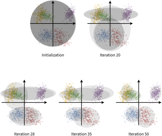
The CAVI algorithm on a Gaussian mixture model, for a dataset of 2D points from five color-coded clusters: the initialization and the variational factors after 20, 28, 35 and 50 iterations. The ellipses are 2σ contours of the variational approximating factors. The figure uses the multivariate (2D) version of the model; the derivation above uses univariate Gaussians. Adapted from: Variational Inference: A Review for Statisticians
The picture above shows that the Gaussians start near the center of the dataset, with a wide variance, and, as the iterations progress, each one moves towards a cluster and narrows around it.