AI Supercomputing: Levels of Parallelism, Linear Regression, Deep Neural Nets and Convolutional Neural Nets
Machine Learning is driven by non-linear optimization models that build an approximator that learns from data. With time, the size and complexity of the data increases, due e.g. to higher-resolution photos, larger text databases, higher number of observable features on input datapoints, etc. The computing power available tends to follow, or somehow adapt, as observed by Moore’s law. However, in msny situations, the amount of data or a large ML model size leads to a problem that does not fit on a regular processor (typically due to insufficient memory), or leads to a very high training time. This is where AI Supercomputing comes to help.
AI Supercomputing focuses on how to distribute data (models, inputs) and computation across several compute units a.k.a processors. The goal is to make the learning problem fit the compute resources, by distributing data and parameters and parallelizing computation. The optimal assignment of data, model parameters and computation to the existing compute and memory resources is a hard problem. The ideal algorithm is characterized as the one that exhibits:
- homogeneous distribution of data across memory units, i.e. balanced memory usage, ideally without data repetitions;
- homogeneous amount of computation assigned to each compute unit, i.e. balanced computation;
- a minimal amount of communication across memory/compute units, or ideally a zero-communication overhead if overlaping of communication and computation is possible; and
- linear or super-linear scaling of the execution time of the algorithm based on the number of precessors. This means that, by increasing (e.g. doubling) the compute resources, we would decrease (halve) the computation.
In practice, guaranteeing these properties is very hard in complex problems (particularly the perfectly-linear scaling), but a good solution can be achieved by cleverly designed algorithms. Let’s start with the basics.
Linear Regression and Mutual Exclusion
Take a simple example of linear regression with input variables \(x\), labels \(y\), learnt weights \(w\) and a loss function set as the Mean Absolute Error. We want to minimize:
\[\begin{align*} MAE(w) = \frac{1}{N} \sum_{n=1}^N | y_n - f(x_n) | \text{, where } f(x_n) = \sum_{j=1}^{M} w_j x_j \end{align*}\]To speed-up the solution, we can parallelize both sums in \(MAE\) and \(f(x_n)\) with several compute units (let’s say \(T\) compute threads) and decompose the computation as:
\[\begin{align*} MAE(w) & = MAE (w_{thread_1}) + MAE (w_{thread_2}) + ... + MAE (w_{thread_T})\\ & = \sum_{n=1}^{\lfloor N/T \rfloor} |y_n - f(x_n)| + \sum_{n=\lfloor N/T \rfloor +1}^{2\lfloor N/T \rfloor} |y_n - f(x_n)| + ... + \sum_{n=(T-1)\lfloor N/T \rfloor +1}^{N} |y_n - f(x_n)| \end{align*}\]This operation is memory-safe for \(f(x_n)\), but unsafe for \(MAE(w)\). In practice, computing \(f(x_n)\) requires a sum of \(M\) independent products written on distinct indices of \(x\), while the final value holding \(MAE(w)\) yields a race condition due to value that needs to be updated with the value of every term \(\|y_n - f(x_n)\|\). What happens to the execution time and final value when several threads try to write simultaneously to the memory space holding it? Let’s study four alternative implementations:
- base case: no parallelism, i.e. use only a single thread. The output is correct but its computation is slow. This implementation is available in AI_SC_1.cpp;
- each thread updates the MAE sum, at every update of the term \(\mid y_n - f(x_n)\mid\). This implementation provides an almost-linear scaling of computation (there’s some overhead on initiating threads). However the output is wrong as several memory corruptions occur when multiple threads try to update the final value (or its memory position) at the same time (AI_SC_2.cpp);
- same as before, however we add a mutex (mutual exclusion) control object. A mutex allows for a section of the code to be locked by a thread, in such way that no other thread can enter it until the first thread has unlocked it. This method gives an accurate result, however it is very slow, due to the waiting time introduced by the mutex (AI_SC_3.cpp);
- finally, we try the same as before, but we compute the sums of each thread independently and perform a single concurrent memory update of the final variable once, and only at the end of the execution. This approach gives the correct result with an almost-linear scaling of the algorithm (AI_SC_4.cpp);
These examples give us three important message: (1) concurrent updates are computationally expensive; (3) parallelization is worth it; and (3) matrix-vector multiplications and updates (that underlie most operations in Machine Learning) can be performed efficiently when individual contributions from compute units are decomposed, computed independently and reduced at the end.
Concurrent access is a big performance issue for some problems, and not all ML problems can be linearly-parallelizable without losing determinism in results. A common example is any method based on random number generation, such as Markov chain Monte Carlo (MCMC). In such scenarios, where compute units draw random number(s) for every datapoint, we either have a central random generator that is concurrently accessed by all threads (reproducible but slow), or a random number per compute unit (efficient, but deterministic only across runs with the same processor count).
From CPU to GPU and TPU/IPU
The spectrum of possible hardware across processors is wide. To name a few, CPUs (Central Processing Units) are high frequency processors with relatively small core count optimized for serial tasks; GPUs (Graphics Processing Unit) are low latency, high core count processors with high vectorization, designed for parallel tasks such as graphics processing or algebraic operations; and most recently IPU/TPUs (Inteligent/Tensor Processing Units), a highly parallel, highly vectorizable processor, with a reduced instruction set and hardware design that is specific to ML.
There are three main aspects that drive the design of processors: power consumption, heat dissipation and temperature. In practice, it is a trade-off problem. As an exmaple, to increase the clockspeed we can reduce the transistor size thus inserting more transistors in the same chip or placing them more tightly in the same area. This leads to an increase of power comsumption and temperature that grows exponentially with the linear decrease in the processor size.
Therefore, for a simillar throughput, many cores of low clock frequency yield the same results of few cores of high frequency, yet at a much lower power comsunption. Equivalently, For a fixed power consumption, one can extract more compute power from many low frequency cores than from a few high frequency cores.

Exponential increase of power comsumption (y axis) for a linear increase of processor frequency (x axis), for processor with one to four cores (colour coded) of the Samsung Exynos 7420 processor. (source: AnandTech)
Looking at the previous plot, we see that, to efficiently maximize GHz/FLOPs throughput, one is much more efficient by having several processors of low clock frequency, instead of fewer of a higher frequency. This explains why GPUs tend to be the preferred choice to compute Machine Learning training problems. And this phylosophy led to the creation of TPUs and IPUs, that explore this trade-off of number of cores vs clock-frequency, with lower-precision floating point representations (to maximize MIMD). Let’s check the common CPU, GPU, and IPU specifications for processors used in compute clusters dedicated to ML tasks:
| cores x clock-frequency \(\hspace{1cm}\) | FLOPs (32 bits representation) \(\hspace{1cm}\) | Max RAM | |
|---|---|---|---|
| Intel Xeon 8180 \(\hspace{1cm}\) | 28x 2.5 Ghz | 1.36 TFLOPS | 768 GB |
| Tesla K80 | 4992x 0.56 Ghz | 8.73 TFLOPS | 2x 12GB |
| Graphcore IPU | 1216 x 1.6Ghz [1] | 31.1 TFLOPS | 304 MiB [2] |
Looking at the previous table, we notice that memory bandwidth increases from CPU to GPU to IPU, however its total capacity is reduced. In practice, small memory is compensated by a very low latency between processor and memory, allowing onloading of offloading of large datasets more efficiently. So how do we train large models when the memory available is too small for the problem representation?
CPU offloading (virtual DNNs)
A common technique to handle memory limitations is CPU offloading, sometimes referred to as virtual Deep Neural Networks. The main goal of this method is to dynamically move to the GPU the portions of data and model that are required for the current and following subset of computation steps, and keep the remaining steps on the CPU.
Take this example of training of a multi-layer Deep Neural Network. We’ve seen on a previous post about DNNs that the output \(x\) for a given layer \(l\) of the network, is represent as:
\[x^{(l)} = f^{(l)} (x^{(l-1)}) = \phi ((W^{(l)})^T x^{(l-1)})\]where \(\phi\) is the activation function. The loss is then computed by taking into account the groundtrugh \(y\) and the composition of the ouputs of all layers in the neural network, ie:
\[L = \frac{1}{N} \sum_{n=1}^N | y_n - f^{(L+1)} \circ ... \circ f^{(2)} \circ f^{(1)} (x_n^{(0)}) |\]The important concept here is the composition of the \(f\) function throughout layers. In practice one only needs the current layer’s state and previous layer output to perform the computation at every layer. This concept has been explored by the vDNN (Rhu et al.) and vDNN+ (Shiram et al) implementations:

An overview of the vDNN(+) implementation on a convolutional neural network. Red arrays represent the data flow of variables \(x\) and \(y\) (layers input and output) during forward propagation. Blue arrows represent data flow during backward progagation. Green arrows represent weight variables. Yellow arrows represent the variables workspace in cuDNN, needed in certain convolutional algorithms. Source: vDNN (Rhu et al.)
For offloading to be possible, we’d ideally want a low latency connectivity between the processor and memory, to allow onloading and offloading to be done with a short communication time. To reduce the waiting time on pushing and pulling a layer to/from the GPU, a viable optimization is to overlap computation and communication, and copy the next layer to be computed while computing the current layer’s update. This way, when the algorithm has finished computing a given layer, it can proceed immediately to the next one as it is already available in memory, thus removing the waiting time on the onloading step.
Let’s look at the offloading algorithm. We start with the forward pass. Looking at the initial formulation of \(x^{(l)}\), we can isolate which variables are used during the forward pass of a given layer. For the computation of the output of a given layer, we need the weights of the neurons in the current layer (\(W^{(l)}\)) and the outputs of neurons on the previous layer \(x^{(l-1)}\). Therefore, for a given layer, the forward pass is represented as:

The forward pass on the vDNN(+) implementation on convolutional neural networks. Data not associated with the current layer being processed (layer N) are marked with a black cross and can safely be removed from the GPU’s memory. Input variables are \(x^{(l-1)}\) (represented as X) and \(W^{(l)}\) (as WS). Source: vDNN (Rhu et al.)
The backward propagation phase is trickier. Referring to the same DNN post, we have represented the derivative of the loss of a given neuron \(j\) in a given layer \(l\), on the input \(z^{(l)} = (W^{(l)})^T x^{(l-1)}\) as \(\delta_j^{(l)}\), where:
\[\delta_j^{(l)} = \frac{\partial L_n}{\partial z_j^{(l)}} = \sum \frac{\partial L_n}{\partial z_k^{(l+1)}} \frac{\partial z_k^{(l+1)}}{\partial z_j^{(l)}} = \sum_k \delta_k^{(l+1)} W_{j,k}^{(l+1)} \phi '(z_j^{(l)})\]i.e., for the backward propagation, we require both the input variable \(x^{(l-1)}\) (inside \(z_j^{(l)}\)), the weights \(W^{(l+1)}\) and the derivatives \(\delta_j^{(l+1)}\). This can now be represented as:
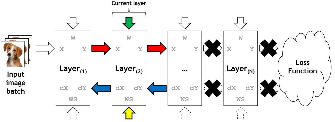
The back propagation phase on the vDNN(+) implementation on convolutional neural networks. Data not associated with the current layer being processed (layer 2) are marked with a black cross and can safely be removed from the GPU’s memory. Input variables are \(x^{(l-1)}\) (represented as X), \(W^{(l+1)}\) (as WS) and \(\delta_j^{(l+1)}\) (as dY). Source: vDNN (Rhu et al.)
Gradient Accumulation and Microbatching
Gradient accumulation is a technique that allows for large batches the be computed, when normally this would be prohobitive due to high memory requirements. The rationale is to break the mini-batch into micro-batches and use the averaged loss and gradient updates at the end of all micro-batches to update the model. The algorithm is as follows:
- At runtime, divide each minibatch in equal subsets of “microbatches”;
- Pass each subset iteratively to the model, compute the forward pass and backpropagation, and compute the gradient updates of that microbatch (without updating the weights);
- Take the average of all the gradients across all processors as the final gradient of the minibatch;
- Use that gradient to do the weights update;
Distributed Data Parallelism
Distributed Data Parallelism (DDP) refers to the family of methods that perform parallelism at the data level, i.e. by allocating distinct mini-batches of data to different processors. The rationale of DDP is simple:
- a copy of the model is instantiated on every processor equally, ie all processors have the same random seed and initiate weights similarly;
- the input dataset is distributed across all processors, by delegating different subsets of data to each processor;
- at the end of each forward pass, gradients are computed for each processor and averaged across all processors, to be used to compute the weight update. This happens at every layer and keeps all models in synchrony after every backward pass.

An illustration of DNN data parallelism on two processors \(p0\) and \(p1\) computing a dataset divided on two equally-sized “batches” of datapoints. Execution of both batches occurs in parallel on both processors, containing each a similar copy of the DNN model. The final weight update is provided by the averaged gradients of the models.
The main advantadge of this method is the linear increase in efficiency, i.e. by doubling the amount of processors, we reduce the compute time by half, minus the communication overhead. However, it’s not memory efficient, since it requires a duplication of the entire model on all compute units, i.e. increasing number of processors allows only for a speedup in solution, not on the increase of the model size.
As a final note, DDP doesn’t always guarantee a deterministic solution independent of the processor count. To guarantee a single communication step per epoch, some operations such as layer normalization are performed locally (at a processor level) leading to a weight update that changes with the data assigned per processor.
For a thorough analysis of the topic, take a look at the paper Measuring the Effects of Data Parallelism on Neural Network Training (Google Labs, arXiv)
Pipeline Parallelism (G-Pipe, PipeDream)
Take the previous neural network with 4 layers stored across a network of processors (here also labelled as workers). If we allocate a worker to each layer (or to a sequence of layers) of the network, we reduce the memory consumption by a factor close to 4. However, traininig now requires a pipeline execution where the activations of the layer in a worker must be communicated to the worker holding the following layer. This method is called pipeline parallelism. A timeline of the execution could then be represented as:

Left-to-right timeline of a serial execution of the training of a deep/convolutional neural net divided across 4 compute units (Workers). Blue squares represent forward passes. Green squares represent backward passes and are defined by two computation steps. The number on each square is the input batch index. Black squares represent moments of idleness, i.e. worker is not performing any computation. Source: PipeDream: Generalized Pipeline Parallelism for DNN Training (Microsoft, arXiv)
We notice that most of the available compute time is spent doing nothing. This is due to the data dependency across layers, mentioned above: one worker can only proceed with the forward (backward) pass when the worker with the previous (next) index has finished its computation and communicated the required activations (weights derivative). A better implementation can be done by feeding to the neural network a sequence of micro-batches. At every iteration, a worker performs a forward (backward) pass on a single data sample and passes the relevant data to the worker holding the following (previous) layer of the network. As soon as that sample is passed, it can immediately start processing the next sample without waiting for the backward propagation of the previous sample to end. This is then equivalent to gradient accumulation with a number of steps equivalent to the number of sequential samples - microbatches - passed per loop. This approach is detailled on the paper GPipe: Efficient Training of Giant Neural Networks using Pipeline Parallelism (Google, 2018, ArXiv) and can be illustrated as:

A pipeline execution with gradient accumulation, computed as a sequence of forward passes on several micro-batches, followed by a backward phase of all micro-batches in the same group. Image source: PipeDream: Generalized Pipeline Parallelism for DNN Training (Microsoft, arXiv)
There are two downsides to the previous method. At first, the activations of every layer need to be kept throughout the whole micro-batch processing, as they are required to perform the backward pass. This leads to high memory requirements. Tp overcome it, there are two possible solutions:
- activation offloading stores and loads the activations to/from the CPU as needed;
- activation checkpointing deletes from memory the activations of every layer as soon as they are communicated to the next processor, and recompute them during backpropagation when needed.
As a second downside, there are till periods of idleness that are impossible to remove. To overcome it, a method based on versioning of activations and updates has been detailed in PipeDream: Generalized Pipeline Parallelism for DNN Training (Microsoft, arXiv). The main idea is overlap forward and backward pass parameters of different mini-batches and micro-batches, and distinguish them with a flag of the mini and micro-batch they belong to. In practice:
- the forward pass of a micro-batch are allowed to start start when the worker is idle, even if the previous micro-batch backward step has not finished;
- whenever a worker is allocated a backward pass of a given mini- and micro-batch, it picks from memory the activations that refer to that mini-batch and micro-batch and performs gradient updates based on that;
- in the event that a worker is allocated a forward pass and a backward pass at the same time, it prioritizes the backward pass in order to reduce max memory consumption.
The following workflow illustration provides an overview of the algorithm:

A pipeline execution of a sequence of batches using the PipeDream strategy. Several forward passes can be in flight, even if they derive from different micro-batches. Backward passes are prioritized over forward passes on each worker. Implementation details and image source: PipeDream: Generalized Pipeline Parallelism for DNN Training (Microsoft, arXiv)
Where’s the caveat? In practice, mixing forward and backward passes from different mini-batches lead to wrong weight updates. Therefore, the authors perform also versioning of the weights, effecticely having several version of the same weights in the model. Therefore, the forward passes use the latest version of the model layers, and the backward may use a previous version of the model activations and optimizer parameters to compute the gradients. This leads to a substantial increase in memory requirements.
Tensor-parallelism
Tensor parallelism is another method for parallelism where the data being distributed across different processors is not the batch dimension (as in data parallelim) or model depth dimension (e.g. pipelining), but the activation level instead. The most common application of this method is by vertically dividing and allocating to different accelerators both the input data and model layers, as in:

A representation of tensor parallelism on a fully-connected DNN, on two processors \(p0\) and \(p1\). Input dataset and each layer of the model are divided and allocated to different processors. Red lines represent weights that have to be communicated to a processor different than the one holding the state of the input data for the same dimension.
Looking at the previous picture, we notice a major drawback in this method. During training, the constant usage of sums of products using all dimensions on the input space will force processors to continuously communicate those variables (red lines in the picture). This communication is synchronous and does not allow an overlap with compute. This creates a major drawback on the execution as it requires a tremendous ammount of communication at every layer of the network and for every input batch. Moreover, since the number of weights between two layers grows quadratically with the increase of neurons (e.g. for layers with neuron count \(N_1\) and \(N_2\), the number of weights are \(N_1 * N_2\) ), this method is not used directly on large input spaces, as the communication becomes a bottleneck.
As as important note: there are several alternative ways to store and distribute tensors that allow for less communication cycles. These are based on splitting the matrices along different dimensions so that matrix-matrix products are done locally (in partial multiplication). This is a complex problem, and in reality, out-of-the-box tensor parallelism for any model is an open problem. The state-of-the-art work on the field follows the Megatron-LM paper: Efficient Large-Scale Language Model Training on GPU Clusters.
Overcomming the communication bottleneck
To reduce the effects of the previous communication overhead, Megraton-LM uses a very simple technique to reduce the ammount of communication. On an MLP block, take the output of each block as \(Y = GeLU(XA)\):
- the typical approach is to split the weight matrix \(A\) along its rows and the input matrix \(X\) along its columns as (for 2 processors \(1\) and \(2\)): \(X=[X_1, X_2]\) and \(A=[A_1, A_2]^T\). This partitioning will result in \(Y = GeLU(X_1A_1 + X_2A_2)\). Since \(GeLU\) is a nonlinear function, \(GeLU(X_1A_1+ X_2A_2) \neq GeLU(X_1A_1) + GeLU(X_2A_2)\) and this approach will require a synchronization point (to sum both partial sums of products) before the \(GeLU\) function.
- the proposed option is to split \(A\) along its columns, i.e. it’s a feature- (not row-) wise partitioning. This allows the \(GeLU\) nonlinearity to be independently applied to the output of each partitioned GEMM: \([Y_1, Y_2] = [GeLU(XA_1), GeLU(XA_2)]\). This removes the synchronization point.
Transformer models follow an analogous approach. For more details, see section 3. Model Parallel Transformers of the Megraton-LM paper for the diagram on Multi-Layer Perceptron and Self-Attention modules.
Intra-layer Parallelism on CNNs
It is relevant to mention that vertical model parallelism has some use cases where it is applicable and highly efficient. A common example is on the parallelism of very high resolution pictures on Convolutional Neural Networks. In practice, due to the kernel operator in CNNs (that has a short spatial span), the dependencies (weights) between two neurons on sequential layers is not quadratic on the input (as before), but constant with size \(F*F\) for a filter of size \(F\).
This method has been detailed by Dryden et al. (Improving Strong-Scaling of CNN Training by Exploiting Finer-Grained Parallelism, Proc. IPDPS 2019). The functioning is illustrated in the picture below and is as follows:
- Input dataset (image pixels) are divided on the height and width dimensions across processors;
- Dependencies among neurons on different dimenstions are limited to the \(F \times F\) filter around each pixel. The weight updates can be computed directly if the neurons in the filter fall in the same processor’s region, or need to be communicated (as before) otherwise. Neurons that need to be communicated are denominated part of the halo region (marked as a violet region in the picture below);
- Similarly to the “CPU offloading (vDNN)” example above, values that need to be communicated are:
- input and weights during forward pass;
- input weights and derivatives during backward pass;
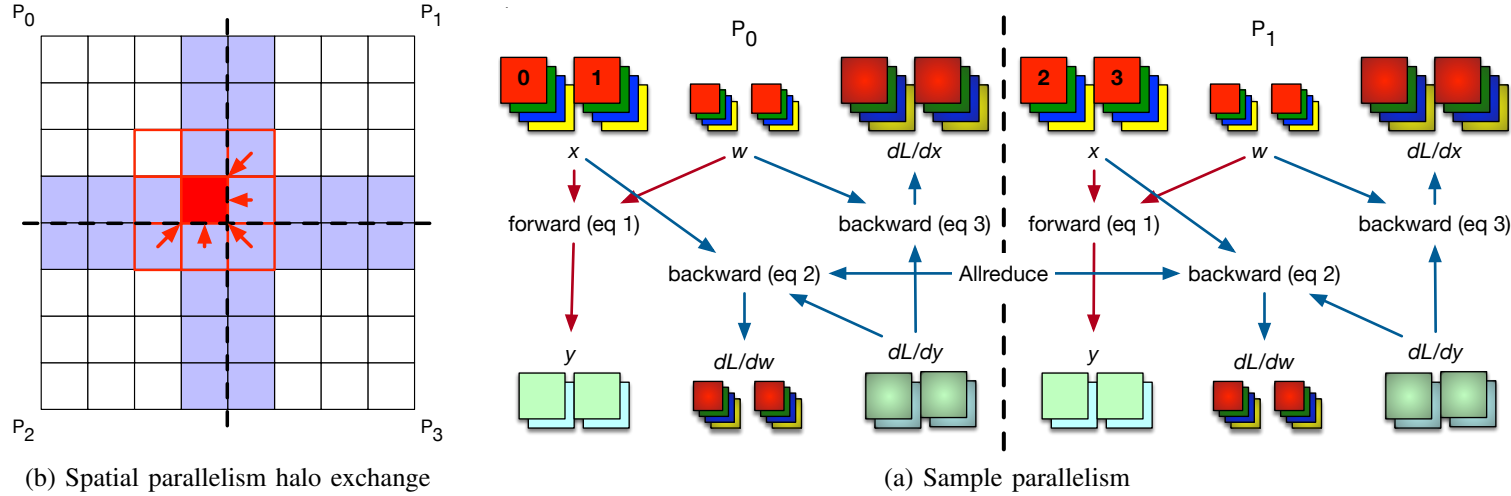
Illustration of model parallelism applied to Convolutional Neural network. LEFT:</b> Parallelism of the pixels of an image across four processors \(p0-p3\). red box: center of the 3x3 convolution filter; red arrow: data movement required for updating neuron in center of filter; violet region: halo region formed of the elements that need to be communicated at every step. RIGHT: communication between processors \(p0\) and \(p1\). Red arrow: forward pass dependencies; blue arrow: backward pass dependencies;
For completion, the equations of the previous picture are the following:
\[y_{k,f,i,j} = \sum_{c=0}^{C-1} \sum_{a=-O}^{O} \sum_{b=-O}^{O} x_{k,c,i+a,j+b} w_{f,c,a+O,b+O}\] \[\frac{dL}{dw_{f,c,a,b}} = \sum_{k=0}^{N-1} \sum_{i=0}^{H-1} \sum_{j=0}^{W-1} \frac{dL}{dy_{k, f, i, j}} x_{k, c, i+a-O, j+b-O}\] \[\frac{dL}{dx_{k,c,i,j}} = \sum_{j=0}^{F-1} \sum_{a=-O}^{O} \sum_{b=-O}^{O} \frac{dL}{dy_{k, f, i-a, j-b}} w_{f, c, a+O, b+O}\]Can you infer the data dependencies displayed in the picture (red and blue arrows) from these equations? We won’t go on details here, but read the original paper if you are interested.
Closing Remarks
We reach the end of this introduction to model parallelism. There’s a class of models that have not been covered: sequence data such as textual sentences. In such cases, the previous techniques can hardly be applied due to the recursive nature of the training algorithm. These topics will be covered in the next post.