AI Supercomputing (part 2): Encoder-Decoder, Transformers, BERT, Sharding, and model compression
In our previous post, we discussed different techniques and levels of parallelism (model, data, pipeline, CPU offloading) and showed that efficient parallelism (with almost-linear scaling) at scale is possible in Machine Learning problems. However, recursive models — such as the ones used in translation and text interpretation tasks — are not easy to parallelize. In this post we explain why.
Encoder-Decoder and Sequence-to-Sequence
The Encoder-Decoder (original paper Sequence to Sequence Learning with Neural Networks (Google, arXiv)) is an AutoEncoder model that learns an encoding and a decoding task applied to two sequences, i.e. it trains for a sequence-to-sequence task such as the translation of a sentence from a given language to a target language. The learning mechanism is a two-phase recursive algorithm, for the encoder and decoder respectively, where each phase is a sequence of iterations over a recursive neural network.
The structure of its Recursive Deep Neural Network (RNN) is as follows:
- Words are past as part of the input, represented by an embedding of dimensionality \(d\);
- The neurons used in the model are not stateless (e.g. like in a regular neuron with an activation function), but have an internal state. Two common examples are Long Short-Term Memory neurons (LSTM) and Gated Recurrent Units (GRU). The set of state variables of the neurons on a single are the layer’s hidden state. In this example, as in most application, we’ll focus on GRU as it includes a single state variable on each neuron (versus two on the LSTM counterpart), making it faster to train;
- The network has three fully connected layers:
- an output layer of size \(h\), whose output value is the embedding of the predicted/groundtruth word;
- a single hiddle layer of size \(d\), refering to the hidden space of the current iteration;
- an input layer of length \(h+d\) (when utilizing GRU neurons) or \(2h+d\) (LSTM), referring to the concatenation of the embedding of the previous iteration’s hidden space (we’ll cover this next), and the embeding of the current word being input. On the first iteration, the input is initialized randomly or with a zero vector;
This structure is easily represented by the following picture:
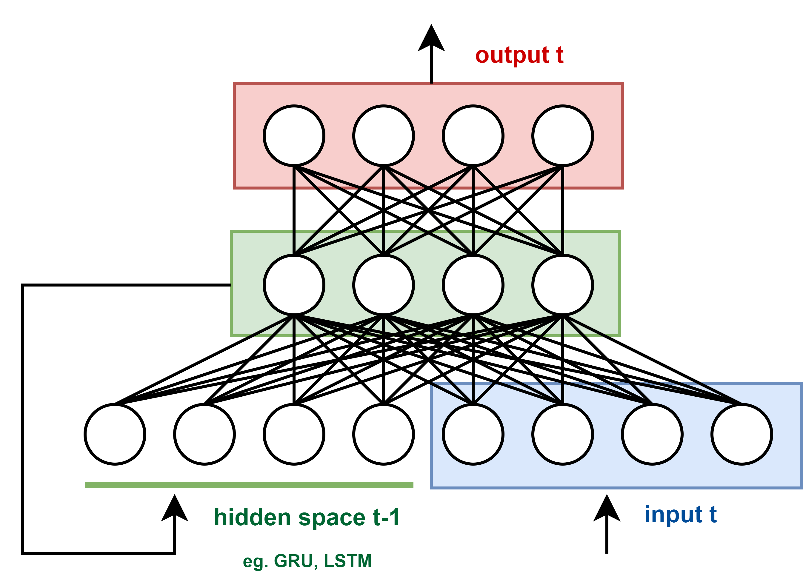
The recursive deep neural network trained on each step of the encoder-decoder architecture. The blue area represent input neurons. The green area represents a single hidden layer formed by the states of the GRU/LSTM neurons of the RNN. The red area represents the model output. The concatenation of the hidden layer of the previous iteration and the current iteration’s input are used as model input.
The training follows with an encoding and decoding phase:
- During the encoding, the RNN processes all the words on the input sequence iteratively, and reutilizes (concatenates) the hidden state of an iteration as input of the next one. The output of the RNN is discarded, as we are simply training the hidden states. When all words have been processed, the hidden state of the RNN is past as input to the first iteration of the decoder;
- The decoder takes on its first step the last encoder’s hidden space and concatenates it with the Beginning of Sentence (BOS) flag (user-defined, usually a vector with only zeros or ones). The output is the first predicted word in the target language. All following steps are simillar: the output and hidden state of a single step is past as input to the next one, and the model can then be trained based on the loss on the output (translated word). The last iteration’s output is the flag End of String (EOS), built similarly to BOS. Training of the RNN iterations happens at every iteration, as in a normal Deep Neural Network.
This algorithm can be illustrated as:

The workflow of an encoder-decoder architecture training by learning the translation of the english sentence “Hello World.” to the Frence sentence “Bonjour le monde.”.
Two relevant remarks about the Encoder-Decoder architecture:
- Once the network is trained, the translation of a new sentence is executed by running encoder iterations until the flag EOS is output;
- An improvement based on the concept of Attention Mechanism delivers improved results by utilising the hidden space of every encoder iteration (not just the last) on the decoding steps, in order to increase the model capatiblities (original paper: Bahdanau et al. Neural Machine Translation by Jointly Learning to Align and Translate);
For the sake of brevity, we will ommit these details and refer you to the Pytorch turorial “NLP from scratch: translation with a sequence to sequence network and attention” if you are curious about the implementation details of regular and attention-based encoder-decoders. Let’s go back to the main subject of this post and the topic of computational complexity.
Parallelism, scaling and acceleration of such sequence-to-sequence models is an issue. There are four main reasons that explain this:
- encoding/decoding is a recursive algorithm, and we can’t parallelize recursive iterations, as each iteration depends on the hidden state of the previous one;
- the DNN underlying the RNN architecture has only a single layer, therefore model parallelism like pipelining (covered in our previous post) won’t provide any gains;
- the hidden layer is composed of \(h\) neurons, and \(h\) is usually a value small enought to allow for acceleration at the layer level (e.g. the model parallelism showned in the our previous post;
- input and output sequences have different lengths, and each batch needs to be a set of input and output sentences of similar lenghts, which makes the batches small and inefficient to parallelize. In practice, some batching is possible by grouping sentences first by length of the encoder inputs, and for each encoder, group by length of decoder inputs. This is however very inneficient as we require an extremmly high number of sentences so that all groups of encoder/decoder pairs are large enough to fully utilize the compute resources at every training batch. Not impossible, but very unlikely.
Transformer
Note: the original Transformer paper is also detailed in the section publications bookmark.
In 2017 the staff at Google introducted the Transformer (original paper Attention is all you need (2017, Google, Arxiv)), overcoming many of the previous issues, while demonstrating better results. The transformer architecture is the following:
![]()
The transformer architecture. Grey regions represent the Encoder (left) and Decoder (right) architectures. Source: Attention is all you need (2017, Google, Arxiv)
The left and right hand side components refer to the encoder and decoder, specifically. We will describe these components in the next sections, and ommit the implementation details to focus on computational complexity. If you’re curious about its implementation, have a look at The Annotated Transformer.
Word and Positional Embeddig
The first unit of importance in the transformer is the embedding unit combined with the positional encoding (red boxes and circles in the previous picture). The transformer model has no recurrence or convolution, so we need a positional encoder to learn the context of a sequence based on the order of its words. Without it, it can only learn from the input as a set of values, not as a sequence, and inputs with swapped tokens would yield the same output. According to the paper, the embedding position \(d\) of a given word in the position \(pos\) of a sentence is:
- \(PE_{(pos,2i)} = sin\left(\frac{pos}{10000^{2i/d}}\right)\) for an even position \(d\) and
- \(PE_{(pos,2i+1)} = cos\left(\frac{pos}{10000^{2i/d}}\right)\) otherwise.
In practice, the embedding is given by the \(sine\) and \(cosine\) waves with a different frequency and offset for each dimension. As an example, for a word with positioning \(pos\) (x axis), then the values at dimensions \(4\), \(5\), \(6\) and \(7\) is:
![]()
The output of the positional encoding in the transformer architecture, for dimensions 4 to 7 of the embedding array, for a word with a sentence-positioning related to the x axis. Source: The Annotated Transformer
Attention Mechanism
The main component of the transformer is the attention mechanism, that determines how the words in input and output sentences interact. In brief, it’s the component that learns the relationship between words in such a way that it learns the relevant bits of information on each context (thus the naming Attention mechanism). The transformer architecture includes not one, but several of these mechanisms, executed in parallel, to allow the model to learn multiple relevant aspects of the input. This Multi-head Attention Mechanism solves for \(n\) heads, What part of the input should I focus on?
Let’s look at a single head of attention mechanism for now. Take the sentence of length \(N\) words, how is each word related to every other word on that sentence? The output of a single attention mechanism is then the \(N \times N\) matrix storing these inter-word importance metric. Here’s an example:
![]()
The attention mechanism output. For the sentence of length \(N=4\) “The big red dog” the output at every row of the attention matrix is the normalized relevance metric of that word to every other word in the sentence. Source: unknown.
How does this mechanism work? According to the paper, each attention head is formulated as:
\[Attention(K, V, Q) = A \, V = softmax\left( \frac{QK^T}{\sqrt{D^{QK}}} \right) V\]Where:
- \(Q\) is a tensor of queries of size \(N^Q×D^{QK}\)
- \(K\) is a tensor of keys of size \(N^{KV}×D^{QK}\), and
- \(V\) is a tensor values of size \(N^{KV}×D^V\), thus
- \(Attention(K,V,Q)\) is of dimension \(N^Q×D^V\).
The tensor \(A\) is the attention score where \(A_{q,k}\) is computed for every query index \(q\) and every key index \(k\), as the argmax of the softmax (softargmax), of the dot products between the query \(Q_q\) and the keys:
\[A_{q,k} = \frac{ \exp \left( \frac{1}{\sqrt{D^{QK}} } Q^{\intercal}_q K_k \right) }{ \sum_l \exp \left( \frac{1}{\sqrt{D^{QK}}} Q^{\intercal}_q K_l \right) }\]The term \(\frac{1}{\sqrt{D^{QK}}}\) helps keeping the range of values roughly unchanged even for large \(D^{QK}\). For each query, the final value is computed for as a weighted sum of the input values by the attention scores as: \(Y_q = \sum_k A_{q,k} \, V_k\).
![]()
The attention operator can be interpreted as matching every query \(Q_q\) with all the keys \(K_1, ..., K_{N^{KV}}\) to get normalized attention scores \(A_{q,1},...,A_{q,N^{KV}}\) (left), and then averaging the values \(V_1,...,V_{N^{KV}}\) with these scores to compute the resulting \(Y_q\) (right). Source: the little book of deep learning.
Notice that in the transformer diagram, each attention module has three inputs (arrows) referring to these three variables. The attention mechanism at the start of each encoder and decoder is retrieving keys, values and queries from its own input, learning the context of the source and target languages, respectively. However, in one occurence of the attention mechanism, the keys and values are provided by the encoder, and the query by the decoder, relating to the module that is trained for the translation at hand.
Finally, the multi-head attention mechanims combines all attention mechanism modules, and is defined as:
\[MHA(K, V, Q) = [head_0,.., head_n]W^{MHA} \,\text{ and }\, head_i = Attention(KW^K_i, VW^V_i, QW^Q_i)\]I.e. it’s a concatenation of all attention heads, and the parameters learnt are the weights of the keys (\(W^K_i\)), values (\(W^V_i\)) and query (\(W^Q_i\)) space of each head \(i\), and a final transformation of the multi-head concatenation \(W^{MHA}\). In terms of computational complexity, the attention mechanism on the encoder is trained on the complete input sequence at once (as illustrated in the “the big red dog” example), instead of looping through all words in the input sequence. Therefore, the attention mechanism replaces the recursive (RNN) iterations on an encoder, by a set of matrix-vector multiplications.
The Masked Multi-head Attention component on the decoder is similar to the regular MHA, but replaces the top diagonal of the attention mechanism matrix by zeros, to hide next word from the model. Decoding is performed with a word of the output sequence of a time, with previously seen words added to the attention array, and the following words set to zero. Applied to the previous example, the four iterations are:
![]()
Input of the masked attention mechanism on the decoder for the sentence “Le gros chien rouge”. The algorithm performs four iterations, one per word. Attention is computed for every word iterated. The mask component of the attention mechanism refers to replacing (in the attention matrix) the position of unseen words by zero. Source: unknown.
Other components
The other components on the transformer are not unique, and have been used previously in other machine learning models:
- The Feed Forward is a regressor (single hidden-layer DNN) that transforms the attention vectors into a form that is valid as input to the decoder or to the next computation phase;
- The Linear transformation component on the decoder expands the space into an array of size equals to the target vocabulary (French in the example);
- The Softmax operation transforms the output of the previous layer into a probability distribution. The word with the highest probability is picked as output;
Computational Complexity
Besides the great reduction in the number of iterations on the encoder size, the authors compare the computational complexity of four comparative models:
![]()
Comparative table of computational complexity of four different learning models. Key: \(n\): sequence length, \(d\): representation dim., \(k\): kernel size; \(r\): size of neighbourhood. Source: Attention is all you need (2017, Google, Arxiv)
For the RNN used in previous Sequence-to-Sequence mechanism, the number of operations performed is in the order of \(d^2\) multiplications (multiplication of weights in a fully-connected layer of a DNN) for each of the \(n\) words in the sentence, therefore \(O(n^2 d)\). On the self-attention mechanism that we discussed in the Transformer, we have several operations of the attention matrix \(n^2\) and the key and query vectors of embedding size \(d\), therefore yielding a complexity of \(O(n d^2)\).
The claim is that the \(O(n^2 d)\) is better than \(O(n d^2)\). This sound illogical in most Machine Learning problems as typically the input size is way larger than the dimensionality of the embedding. However, remember that \(n\) here is the number of words in a sentence (in the order of \(n \approx 70\)) and \(d\) is the size of the embedding (\(d \approx 2000\)).
To summarize, the encoder-decoder architecture of the transformer allows a faster non-recursive training of input sequences, and a faster training of output sentences, making it much more efficient than the sequence-to-sequence approaches discussed initially.
BERT: Bidirectional Encoder Representation from Transformers
Note: the original BERT paper is also detailed in the section publications bookmark.
Attending to the previous topic, the main rationale of the Transformer’s Encoder-Decoder is that:
- The encoder learns the context of the input language (English in the previous example);
- The decoder learns the task of the input-to-output languages (the English-to-French translation);
So, the encoder is efficiently trained and learns a context. So the main question is “Can we use only the Encoder’s context and learn complex tasks?”. This led to the introduction of the BERT model (original paper BERT: Pre-training of Deep Bidirectional Transformers for Language Understanding, Google AI). BERT is a stack of Transformer encoders that Learns language contexts and performs interpretation tasks.

The BERT model, as a stack of Transformer encoders.
The training is performed in two phases. A pre-training phase learns the contexts of the language. And a fine-tuning phase adapts the trained model to the task being solved. Let’s start with the pre-training.
Pre-training
The pre-training phase is based on the simultaneous resolution of two self-supervised prediction tasks:
- Masked language model: given a sentence with works replaced with a flag (or masked), train it against the same sentence with those words in place;
- Next sentence prediction: Given two sentences, train the model to guess if the second sentence follows from the first or not;
Example of two training examples:
Input = [CLS] the man went to [MASK] store [SEP] He bought a gallon [MASK] milk [SEP]
Output = [IsNext] the man went to the store [SEP] He bought a gallon of milk [SEP]

Input = [CLS] the man [MASK] to the store [SEP] penguins [MASK] to jump [SEP]
Output = [NotNext] the man went to the store [SEP] penguins like to jump [SEP]
Note that the Yes/No flag related to the second task is past as the first embedded word in the output. The layout of the input data is:
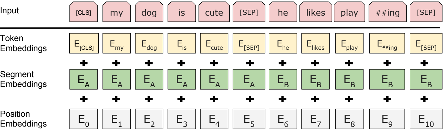
The input of the BERT model. Position Emdebbings are similar to the transformer model, discussed above. Segment embeddings flag each word as part of the first or second sentence. Token embedding are the text-embeddings of the input data. The datapoint being input to the model is the concatenation of these three embeddings. Source: Attention is all you need (2017, Google, Arxiv)
As a side note, the authors trained this model on BooksCorpus (800M words) and English Wikipedia (2,500M words), using 24 BERT layers, batches of 256 sentences with 512 tokens each.
Fine-tuning
The fine-tuning phase adds an extra layer to the pre-trained BERT model, in order to train the model to the task at hand. This approach has been applied previously in other models, particularly on Convolutional Neural Nets, where the first layers are pre-trained and learnt edges and lines, and the remaining layers are added later and used on the training of the object-specific detection.
In the original paper, the authors demonstrated this model successfully being applied to four families of tasks:
- Sentence Pair Classification Tasks: classification of context from pairs of sentences. Examples: do sentences agree/disagree, does the second sentence follow from the previous one, do they describe a simillar context, etc. Similarly to the pre-training phase of the BERT models, the label is past as the first embedded symbol of the output;
- Single Sentence Classification Tasks: similar to the previous, but applied to a single sentence. Used for learning contexts like finding hateful speech, etc.;
- Question Answering Tasks: allows one to pass as input the concatenation of the question and a paragraph where the answer to the question is available. The output of the model is the input with the embeddings representing the start and end word of the answer replaced by a marker. As an example:
- input: “[CLS] His name is John. John is a Swiss carpenter and he is 23 years old [SEP] How old is John”;
- output: “[CLS] His name is John. John is a Swiss carpenter and ###he is 23 years old### [SEP] How old is John”;
- Single Sentence Tagging tasks: retrieves the classes of individual words e.g. Name, Location, Job, etc, by replacing each relevant word with its class id. As an example:
- input: “[CLS] His name is John. John is a Swiss carpenter and he is 23 years old”;
- output: “[CLS] His name is [NAME]. [NAME] is a [NATIONALITY] [OCCUPATION] and he is [AGE] years old”.
The input and output models of the fine-tuning of these tasks are illustrated in the following picture:
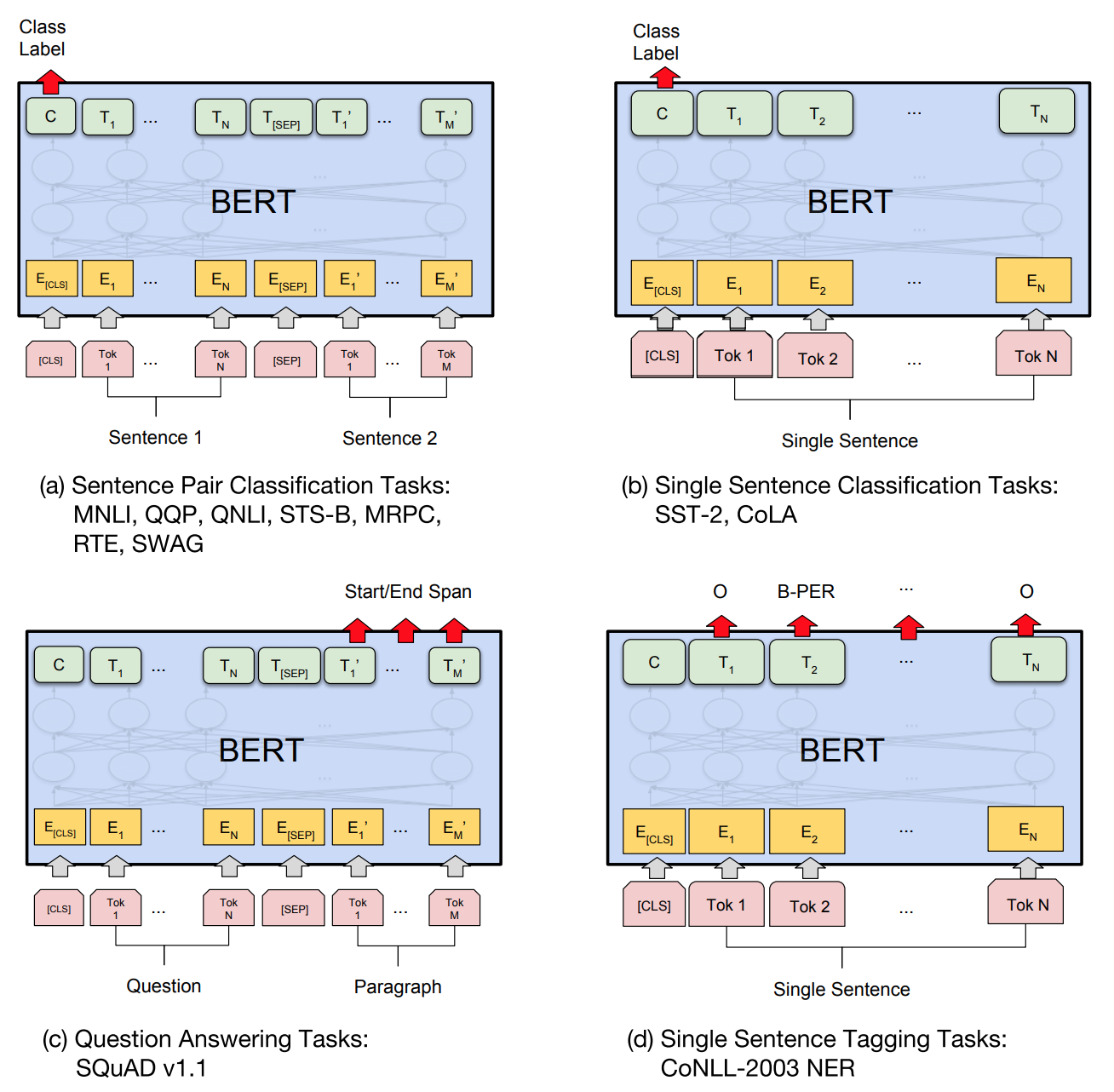
Input and output of the fine-tuning phase of a BERT network, applied to four different interpretation tasks. Source: Attention is all you need (2017, Google, Arxiv)
As a final note, information encoded by BERT is useful but, on its own, insufficient to perform a translation task. However, “BERT pre-training allows for a better initialization point for [an] Neural Machine Translation model” (source: Clichant et al.,On the use of BERT for Neural Machine Translation, arXiv).
Sharding
The limits of supercomputing in Machine Learning can been pushed to a far greater extent by combining several of previous approaches. As an example, one can combine Distributed Data Parallelism, Pipeline parallelism and gradient accumulation to achieve larger compute parallelism (shorter runtime), a larger model, and a larger batch size.
On top of that, when using model parallelism such as pipelining, each processor can keep only the subset of model layers that it needs for its computation. In practice, the optimizer parameters and temporary buffers that each processor holds in memory refer only to the computation it is required to do. The model weights can also be divided the same way — even though they have a much smaller memory footprint — sacrificing memory reduction for a larger runtime. In this scenario, processors continuously communicate the activation and gradients (forward and backward passes) to the processors holding connecting layers in the network. This can also be combined with data parallelism, leading to a setup where each processor has a subset of the data batch and a subset of the model. This technique is called Sharding, where a shard is a subset of the model layers that is delegated to individual compute units. If you are interested in this topic, see ZeRO and DeepSpeed work at Microsoft ( Turing-NLG blog post, www.deepspeed.ai/, ZeRO paper), the Megatron work at NVIDIA and the GPT work at OpenAI.
Let’s take a look at the particular sharding implementation in the paper ZeRO: Memory Optimizations Toward Training Trillion Parameter Models, Microsoft. ZeRO (as in Zero Redundancy Optimizer) is a parallelism method that “eliminates memory redundancies in data- and model-parallel training while retaining low communication volume and high computational granularity, allowing us to scale the model size proportional to the number of devices with sustained high efficiency”. The results presented show the (at the time) largest language model ever created (17B parameters), beating Bert-large (0.3B), GPT-2 (1.5B), Megatron-LM (8.3B), and T5 (11B). It also demonstrates super-linear speedup on 400 GPUs (due to an increase of batch size per accelerator). Sharding eliminates several drawbacks in sigle-approach parallelism. As an example, using only model parallelism that splits the model vertically (on each layer), leading to high communication and scaling limitations. Moreover, data parallelism alone has good compute/communication efficiency but poor memory efficiency. In practice, memory consumption of the existing systems on model training and classify it into two parts:
- For large models, the majority of the memory is occupied by model states which include the optimizer states (such as momentum and variances in Adam), gradients, and parameters;
- The remaining memory is consumed by activation, temporary buffers and unusable fragmented memory (residual states).
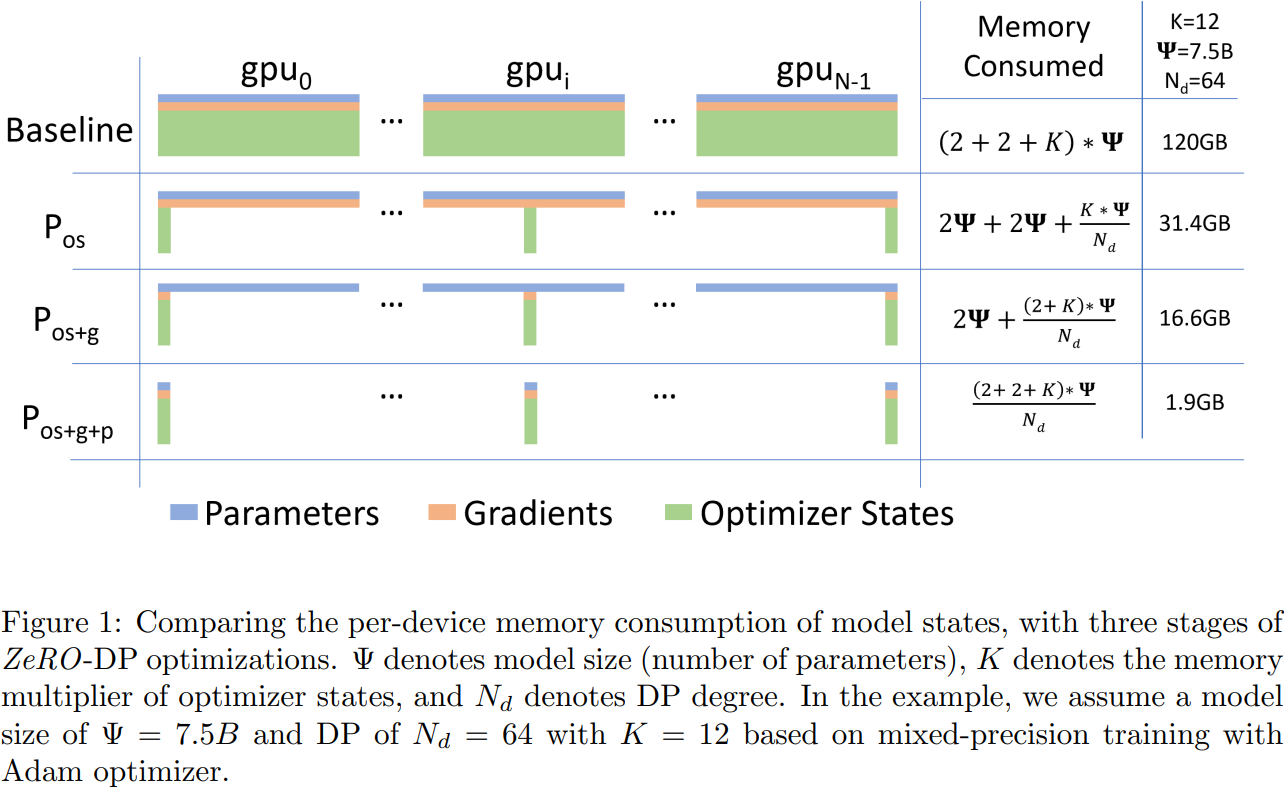
To yield “optimal” memmory usage, ZeRO-DP claims to have the computation/efficiency of Data Parallelism (DP) while achieving memory efficiency of Model Parallelism (MP). This is achieved by three cumulative optimizations: Optimizer State Partitioning (\(P_{os}\), 4x memory reduction and same communication as DP), Gradient Partitioning (\(P_{os+g}\), 8x memory reduction, same comm.) and Parameter Partitioning (\(P_{os+g+p}\), memory reduction linear with number of accelerations \(N_d\), 50\% increase in communication). ZeRO-DP is at least as memory-efficient and scalable as MP, or more when MP can’t divide the model evenly. This is achieved by “removing the memory state redundancies across data-parallel processes by partitioning the model states instead of replicating them, and [..] using a dynamic communication schedule during training. In practice:
- non-overlapping subsets of layers are delegated to different accelerators;
- different optimization levels refer to what content is split or kept across GPUs, as in the figure below;
- content that is not replicated but is instead divided in synchronized with dynamic communication across connecting layers.
Thus, each processor is allocated a subset of data (DP) and a subset of the model (MP). When that data goes through its layers it will broadcast its layers parameters to other accelerators on the forward pass. Each GPU will run its own data using the received parameters. During the backward pass, gradients will be reduced. See bottom figure and video here.
When compared to MP, “Zero-DP has better scaling efficiency than MP because MP reduces the granularity of the computation while also increasing the communication overhead” and “Zero-R removes the memory redundancies in MP by partitioning the activations checkpoints across GPUs, and uses allgather to reconstruct them on demand”. The forward and backward pass schematics are as follows:
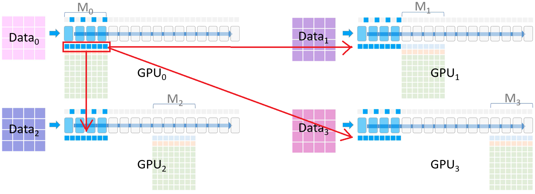
- forward pass: the initial portion of model (\(M_0\)) assigned to \(GPU_0\). It broadcasts its model parameters \(M_0\) to all GPUs (red arrows). Each GPU will do a forward pass of their own data on the received parameters. As we move forward in the model, other GPUs similarly communicate their parameters. The partial activations for each layer are stored by all GPUs. The loss is then computed for each GPU’s data;
- backward propagation: on the first iteration of the Backwards pass, GPUs 0,1 and 2 hold the gradients of the last GPU’s model layers \(M_3\) for data points 0, 1 and 2. Combined with the partial activation stored, the partial gradient updates can be computed locally. An all-reduce of all updates will compute the averaged gradient update for model portion \(M_3\) in \(GPU_3\) (green arrows). All remaining layers follow analogously.
Finally, ZeRO can be complemented with techniques that reduce activation memory such as compression, checkpointing and live analysis. CPU offloading is not recommended or used as “50% of training time can be spent on GPU-CPU-GPU transfers” and this would penalize performance heavily.
Model compression for reduced memory footprint and runtime
Many use cases will require model size to be small for deployment (particularly onto embedded systems), or require inter-layer communication to be small due to storage or network bandwidth limitations, or even benefit from a smaller numerical representation to increase vectorization. To handle that, some commonly used techniques are:
- Pruning methods, where weights or neurons are dropped after training or during training (via a train-prune-train-prune-etc workflow). Note that prunning of weights alone will reduce memory footprint but not compute time in GPUs due to the registers being filled with the same neurons as pre-prunning;
- Quantization methods to reduce the numerical representation, value ranges and bit counts of values. The common use case is to use reduce of mixed floating point representation of values, reducing memory footprint and runtime (by increasing vectorization). Few relevant topics:
- the paper Mixed Precision Training discusses which data types (parameters, gradients, accumulators) required which precision and provides good guidances on mixed precision training.
- a recent floating point representation called bfloat16 (brain floating point), a different 16-bit representation, is important for ML as it represents a wider dynamic range of numeric values than the regular 16-bit representation. This is due to having more bits reserved to the exponent (8 bits, just like 32-bit f.p.) compared to the traditional 16-bit representation (5 bit). In practice, it deliveres the range of a 32-bit representation with the memory consumption and runtime of a 16-bit representation, due to a tradeoff of range vs precision.

- reduced floating point representations (e.g. 16-bit) are commonly combined with (dynamic) loss scaling, a technique that scales up the values of the gradients so that very small gradient values are not represented as zero in the fraction bits of the f.p. representation.
- Knowledge distillation, a special case of model compression, that transfer learning from a larger to a smaller model. This allows the smaller model to be smaller and lighter, and some times of increased performance;
- Checkpointing to avoid storing all activations of intermediate layers — required for back-propagation — in lieu of on-the-fly computation of activations from a previous checkpoint (layer). The ammount of checkpointed layers guides the tradeoff between runtime increase and memory decrease;
- Neural architecture search (NAS), a method to search for the parameters that define the architecture of the models (e.g. number of layers, layer sizes, etc). I have no applied exposure to this method, but found this paper to be very insightful in surveying existing methods;