Deep Neural Networks, backpropagation, autodiff, dropout, CNNs and embeddings
Deep Neural networks – also known as Multi Layer Perceptrons – are universal approximator, i.e. an ML approximator to any function in a bounded continuous domain. They’re the most important and relevant ML tool on the field of supervised learning as they’re included in models related to most supervised tasks.
The structure of a basic NN is the following: one input layer of size \(D\), \(L\) hidden layers of size \(K\), and one output layer. It is a feedfoward network: the computation performed by the network starts with the input from the left and flows to the right. There is no feedback loop. It can be used for regression (when input and output are provided) and for classification (when input are provided and new output is the classifier).

source: Machine Learning lecture notes, M Jaggi, EPFL
Input and output layers work similarly to any previous regression method. Hidden layers are different. The output at the node \(j\) in hidden layer \(l\) is denoted by:
\[x_j^{(l)} = \phi ( \sum_i w_{i,j}^{(l)} x_i^{(l-1)}+b_j^{(l)}).\]where \(b\) is the bias term, trained equally to any other weight. Note that, in order to compute the output we first compute the weighted sum of the inputs and then apply an activation function \(\phi\) to this sum. We can equally describe the function that is implemented by each layer in the form:
\[x^{(l)} = f^{(l)} (x^{(l-1)}) = \phi ((W^{(l)})^T x^{(l-1)}+b^{(l)})\]where \(f\) is the regression function of neurons, as previously. Some popular choices of activation functions are:
- sigmoid function: \(\phi(x) = \frac{1}{1+e^{-x}}\), positive and bounded;
- tanh = \(\phi(x) = \frac{e^x - e^{-x}}{e^x+e^{-x}}\), balanced (positive and negative) and bounded;
- Rectified linear Unit – ReLU: \(\phi(x) = [x]_+ = maxo\{0,x\}\), always positive and unbounded; often used as it’s computationally cheap and helps fighting the issue of decaying weights of DNN as the positive output region does not have a small derivative;
- Leaky ReLU: \(\phi(x) = max \{\alpha x,x\}\). Fixes the problem of dying weights in Non-leaky rectified linear units;
- In brief, if the dot product of the input to a ReLU with its weights is negative, the output is 0. The gradient of \(max\{ 0,x \}\) is \(0\) when the output is \(0\). If for any reason the output is consistently \(0\) (for example, if the ReLU has a large negative bias), then the gradient will be consistently 0. The error signal backpropagated from later layers gets multiplied by this 0, so no error signal ever passes to earlier layers. The ReLU has died. With leaky ReLUs, the gradient is never 0, and this problem is avoided.
Back-propagation
Similarly to previous regression use cases, we are required to minimize the loss in the system, using e.g. Stochastig Gradient Descent. As always when dealing with gradient descent we compute the gradient of the cost function for a particular input sample (with respect to all weights of the net and all bias terms) and then we take a small step in the direction opposite to this gradient. Computing the derivative with respect to a particular parameter is really just applying the chain rule of calculus. The cost function can be written as (details omitted):
\[L = \frac{1}{N} \sum_{n=1}^N ( y_n - f^{(L+1)} \circ ... \circ f^{(2)} \circ f^{(1)} (x_n^{(0)}) ) ^2\]Since in general there are many parameters it would not be efficient to do this for each parameter individually. However, the algorithm of back propagation alows us to do it more efficently. Our aim is to compute:
\[\frac{\partial L_n}{\partial w_{i,j}^{(l)}}, l=1, ..., L+1 \text {, and } \frac{\partial L_n}{\partial b_{j}^{(l)}}, l=1, ..., L+1 \label{eq_gradient}\]For simplicity, we will represent the total input computed at the \(l\)-th layer as
\[z^{(l)} = (W^{(l)})^T x^{(l-1)}+b^{(l)} . \label{eq_z}\]i.e. \(z^{(l)}\) is is the total input computed at layer \(l\) before applying the activation funtion. These quantities are easy to compute by a forward pass in the network, starting at \(x^{(0)} = x_n\) and then applying this recursion for \(l=1,...,L+1\).
Now, let
\[\delta_j^{(l)} = \frac{\partial L_n}{\partial z_j^{(l)}}. \label{eq_delta}\]These quantities are easier to compute with a backward pass:
\[\begin{align*} \delta_j^{(l)} = & \frac{\partial L_n}{\partial z_j^{(l)}} \\ = & \sum_k \frac{\partial L_n}{\partial z_k^{(l+1)}} \frac{\partial z_k^{(l+1)}}{\partial z_j^{(l)}} \\ = & \sum_k \delta_k^{(l+1)} \frac{\partial (W^{(l+1)})^T x^{(l)}+b^{(l+1)}}{\partial z_j^{(l)}} \\ = & \sum_k \delta_k^{(l+1)} W_{j,k}^{(l+1)} \frac{\partial x^{(l)}}{\partial z_j^{(l)}} \\ = & \sum_k \delta_k^{(l+1)} W_{j,k}^{(l+1)} \phi '(z_j^{(l)}) \end{align*}\]We used the chain rule on the second equality operation. Going back to equation \ref{eq_gradient}:
\[\frac{\partial L_n}{\partial w_{i,j}^{(l)}} = \sum_k \frac{\partial L_n}{\partial z_k^{(l)}} \frac{\partial z_k^{(l)}}{\partial w_{i,j}^{(l)}} = \delta_j^{(l)} x_j^{(l-1)} \label{eq_w}\]Here we used the chain rule, equation \ref{eq_delta} on the definition of \(\delta\), and the partial derivative of equation \ref{eq_z} over \(w\). In a similar manner:
\[\frac{\partial L_n}{\partial b_{j}^{(l)}} = \sum_k \frac{\partial L_n}{\partial z_k^{(l)}} \frac{\partial z_k^{(l)}}{\partial b_{j}^{(l)}} = \delta_j^{(l)} \cdot 1 = \delta_j^{(l)} \label{eq_b}\]The complete back propagation is then summarized as:
- Forward pass: set \(x^{(0)} = x_n\). Compute \(z^{(l)}\) for \(l=1,...,l+1\);
- Backward pass: set \(\delta ^{(L+1)}\) using the appropriate loss and activation function. Compute \(\delta ^{(L+1)}\) for \(l = L, ..., 1\);
- Final computation: for all parameters compute \(\frac{\partial L_n}{\partial w_{i,j}^{(l)}}\) (eq. \ref{eq_w}) and \(\frac{\partial L_n}{\partial b_{j}^{(l)}}\) (eq. \ref{eq_b});
Automatic Differentiation
The chain rule shows us the theoretical framework, but not how to compute it efficiently. In practice, contraritly to the back-propagation algorithm above, automatic differentiation (“autodiff”) algorithms such as pytorch’s autograd, do not require the derivatives of the loss and activation functions to be specified explicitly.
Instead, a computational graph (a DAG) is created dynamically, where nodes in the grap are added as modules’ forward are called. The backward propagation will then be computed by performing the chain rule on the derivatives (grad_fn) of the nodes in the computational graph. Recursive calls will add new nodes to the graph for every call, and conditional calls may add different nodes at each forward pass - therefore, the computational graph cannot be extracted from the model definition directly (see an example here). Finally, when the tensor.backward() is called, it will recursively compute the gradients up to the leaf node of the graph. When this process halts, the computational graph will be discarded and a new one may be creating via a new forward call (unless retain_graph=True is set in the backward function). For more details, refer to Chi-Feng Wang’s post for an illustrative example of the automatic differentiation graph, or the Princeton course COS 324 in automatic differentiation for a thorough explanation of the whole process.
Storing a computational graph is also useful for activation checkpointing where one needs to recompute a module’s output during the backward pass. A good example of activation checkpointing based on the reentrant on non-reentrant pytorch implementation can be found in the post How Activation Checkpointing enables scaling up training deep learning models.
Also, it is then logical that inference requires less memory than training, as training requires the computational graph to save all activations. For completeness, a very good notebook that details a step by step overview of the back propagation theory applied to a real example can be found in Hooks for autograd saved tensors and PyTorch Autograd: Backpropagation.
Dropout
Dropout is a method that drops neurons (in different layers) with a given probability \(p\) during train time. For each training minibatch, a new network is sampled. The outputs of the kept neurons are scaled by \(1/(1-p)\). At inference time, all neurons are used, and no dropout is applied. A simple code snippet to explain this is:
class MyDropout(nn.Module):
    def forward(self, X):
        if self.training:
            binomial = torch.distributions.binomial.Binomial(probs=1-self.p)
            return X * binomial.sample(X.size()) * (1.0/(1-self.p))
        return X
Dropout helps reducing overfitting, as the network learns to never rely on any given activations, so it learns redundant ways of solving the task with multiple neurons. It also leads to sparse activations, similar to a regularization (L2). Dropout can be improved by adding max-norm regularization, decaying learning rate and high momentum. Dropping 20% of input units and 50% of hidden units was often found to be optimal in the original publication. It’s computationally less expensive than regular model averaging of multiple trained DNNs. However, it takes 2-3 times longer to train than single fully-connected DNNs because requires way more epochs, as parameter updates are very noisy. Because a fully connected layer occupies most of the parameters, it is prone to overfitting. Therefore, dropout increases model generalization.

Convolutional Neural Networks
The disadvantage of large neural networks is that it has a very high number of parameters so it may require lots of data to be trained. In some scenarios, local training should suffice: e.g. in an audio stream, it is natural to process an input stream \(x^{(0)}[n]\) stream by running it through a linear time-invariant filter, whose output \(x^{(1)}[n]\) is given by the convolution of the input \(x^{(0)}[n]\) and the \(f [n]\), as:
\[x^{(1)}[n] = \sum_k f[k]x^{(0)} [n-k]\]The filter \(f\) is local i.e. \(f[k]=0\), for \(k \ge K\). By choosing an appropriate type of filter we can bring out various aspects of the underlying signal, e.g. we can smooth features by averaging, or we can enhance differences between neighboring elements by taking a high-pass filter. An analogous scenario is visible in case of a picture:
\[x^{(1)}[n,m] = \sum_{k,l} f[k,l]x^{(0)} [n-k,m-l]\]We see that the output \(x^{(1)}\) at position \([n, m]\) only depends on the value of the input \(x^{(0)}\) at positions close to \([n, m]\). So we no longer need a fully connected network but only the one that representes the local strucure, leading to fewer parameters to deal with. This structure implies that we should use the same filter (e.g., not only the same connection-pattern but also the same weights) at every position! This is called weight sharing, drastically reducing the number of parameters further. The difference between a locally/sparse connected and a fully connected is obvious:

It is common to not only compute the output of a single filter but to use multiple filters. The various outputs are called channels. This introduces some additional parameters into the model. If we add several channels we do not end up with a 2D output in the next level but in fact with a 3D output. Per layer we have increasingly more channels but a smaller “footprint.” In brief, applying the local connectivity to a 2D input dataset on a deep neural network, we have the final structure as:
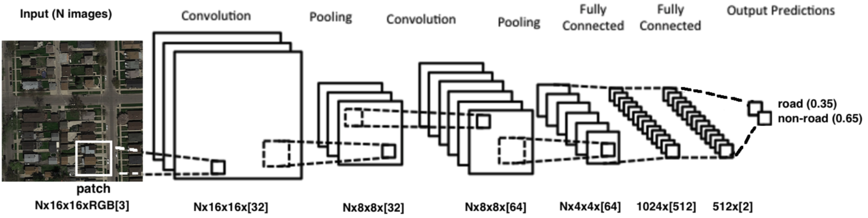
Notice the three types of operations involved:
- convolutional layer: applies a convolution operation to the input, passing the result to the next layer. The convolution emulates the response of an individual neuron to visual stimuli;
- convolution is a mathematical operation on two functions to produce a third function that expresses how the shape of one is modified by the other. Convolution is similar to cross-correlation;
- pooling: combine the outputs of neuron clusters at one layer into a single neuron in the next layer.
- A very common operation is the max pooling, that uses the maximum value from each of a cluster of neurons at the prior layer;
- fully connected: similar to multi-layer perceptron, providing the universal approximator function ;
The size of each picture typically gets smaller and smaller as we proceed through the layers, either due to the handling of the boundary or because we might perform subsampling.
Training follows from backpropagation, ignoring that some weights are shared, and considering each weight on each edge to be an independent variable. Once the gradient has been computed for this network with independent weights, just sum up the gradients of all edges that share the same weight. This gives us the gradient for the network with weight sharing.
Skip connections
An issue with very deep networks is that the performance of the model drops down with the increase in depth of the architecture. This is known as the degradation problem. One possible reason is overfitting: the models tends to overfit if given too much capacity. Other reasons are the vanishing gradients and/or exploding gradients. A way to improve is to use normalization techniques to ensure that gradients have healthy norms.
A better way to improve this is to provide layers of the network with outputs from layers that are not directly connected. These connections will skip some of the layers in the neural network and feed the output of one layer as the input of the next layers — justifying the name skip connections. In practive, the input to a given layer will be the combination (typically via addition or concatenation) of the input of several previous layers.
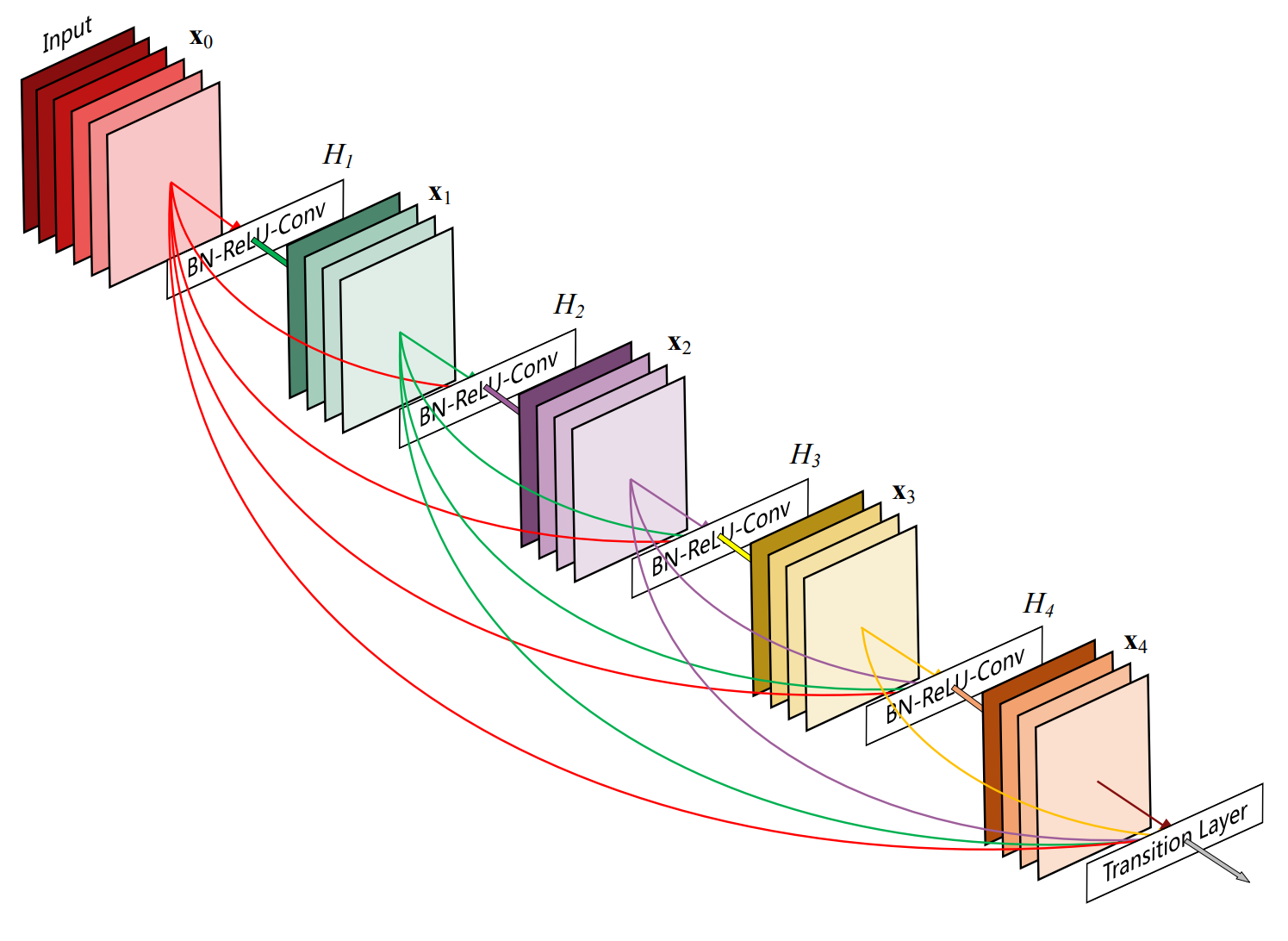
An example of a CNN with skip connections (DenseNet). source: Deep Residual Learning for Image Recognition
There is currently a plethora of different implementations of CNNs with several layouts of skip connections. If you are curious to know more, have a look at ResNet, DenseNet and U-net.
Embeddings
Embeddings in machine learning are dense, low-dimensional vector representations of data (e.g., words, images, or users) that capture their semantic or contextual meaning in a continuous vector space. Embeddings can be collected by passing input data (e.g., text, images) through a trained machine learning model (e.g., a neural network) and extracting the values from a specific intermediate layer, typically before the final output layer.
A list of most common data types and embedding types:
- words: one-hot vectors or Word2vec (skipgram or continuous bag of words)
- skipgram: slower to train (“3 days”), better in capturing better semantic relationships, e.g. for ‘cat’ return ‘dog’ as a word with close embeddings;
- CBOW: faster to train (“few hours”), better syntactic relationships between words, e.g. for ‘cat’ return ‘cats’;
- text (word sequences): BERT
- non-textual sequences: Encoder-Decoders e.g. LSTMs RNNs
- point cluster or array: Principal Component Analysis
- images:
- in a classification task: use the activation of the last layer before the layer that does logit/softmax. I.e. the input to the final layer, i.e. the ouput of the one before last;
- in an image-to-image task e.g. segmentation e.g. using a U-net: use the activation the last downsampling layers which is the first layer of upsampling layers, i.e. the information bottleneck;
- videos: input is now 5D (batch size, time, channels, height, width) where the input is a sequence of video frames stacked on the time dimension. Embeddings are collected similarly to a regular CNN (adapted to use 3D instead of 2D convolutions, etc);
- graphs: embedding of a graph is given by the embedding of a node after several steps of the message passing algorithm as \(x_i^{(k)} = \gamma^{(k)} \left( x_j^{(k-1)}, \Box_{j} \, \phi^{(k)} \left( x_i^{(k-1)}, x_j^{(k-1)}, e_{j,i} \right) \right)\), where:
- \(x_i^{(k)}\) is the embedding of node \(x_i\) at messape passing step \(k\);
- \(e_{i,j}\) is the embedding of the edges between nodes \(i\) and \(j\);
- \(\Box\) is a differentiable, permutation invariant function e.g. sum, mean, max;
- and \(\gamma\) and \(\phi\) are differentiable functions such as DNNs or RNNs (LSTMs, GRUs).