Unsupervised Learning basics and Principal Component Analysis
Unsupervised Learning is the feld of Machine Learning dedicated to the methods of learning without supervision or reward signals. In practice, and contrarily to the fields of Reinforcement Learning and Supervised Learning, the data is the only information provided to the methods. However, methods are still very powerful and are commonly used for applications such as image compression, dimensionality reduction and classification.
Foreword: Hebbian Learning
Among several biologically-inspired learning models, Hebbian learning (Donald Hebb,1949) is probably the oldest. Its general concept forms the basis for many learning algorithms, including backpropagation. The main rationale is based on the synaptic changes for neurons that spike in close instants in time (motto “if they fire together, they wire together”). It is known from the Spike-Timing-Dependent Plasticity (STDP, Markram et al. Frontiers) that the increase/decrease of a given synaptic strenght is correlated with the time difference between a pre- and a post-synaptic neuron spike times. In essence, if a neuron spikes and if it leads to the firing of the output neuron, the synapse is strengthned.
In his own words (Hebb, 1949):
When an axon of cell j repeatedly or persistently takes part in firing cell i, then js efficiency as one of the cells firing i is increased.
Analogously, in artifical system, the weight of a connection between two artificial neurons adapts accordingly. Mathematically, we can describe the change of the weight \(w\) at every iteration with the general Hebb’s rule based on the activity \(x\) of neurons \(i\) and \(j\) as:
\[\frac{d}{dt}w_{ij} = F (w_{ij}; x_i, x_j)\]or the simplest Hebbian learning rule as:
\[\frac{d}{dt}w_{ij} = \eta x_i y_j\]where \(\eta\) is the learning rate, \(y_j\) is the output function of the neuron \(x_j\), and \(i\) and \(j\) are the neuron ids. Hebbian is a local learning model i.e. only looks at the two involved neurons and does not take into account the activity in the overall system. Hebbian is considered Unsupervised Learning, or learning that is acquired only with the existing dataset without any external stimuli or classifier of accuracy. Among others, a common formalization of the Hebbian rule is the Oja’s learning rule:
\[\frac{d}{dt}w_{ij} = \eta (x_i y_j - y_j^2 w_i).\]The squared output \(y^2\) guarantees that the larger the output of the neuron becomes, the stronger is this balancing effect. Another common formulation is the covarience rule
\[\frac{d}{dt}w_{ij} = \eta (x_i - \langle x_i \rangle) ( y_j - \langle y_j \rangle )\]assuming that \(x\) and \(y\) fluctuate around the mean values \(\langle x \rangle\) and \(\langle y \rangle\). Or the Bienenstock-Cooper-Munroe (BCM, 1982) rule:
\[\frac{d}{dt}w_{ij} = \eta y_j x_i (x_i - \langle x_i \rangle )\]a physical theory of learning in the visual cortex developed in 1981, proposing a sliding threshold for Long-term potentiation (LTP) depression (LTD) induction, and stating that synaptic plasticity is stabilized by a dynamic adaptation of the time-averaged postsynaptic activity.
Typically the output of a neuron is a function of a linear multiplication of the weights and the input, as:
\[y \propto g(\sum_i w_{ij} x_i)\]where \(g\) is the pre-synaptic signal function, commonly referred to as the activation function. On the simplest use case of a linear neuron
\[y = \sum_i w_i x_i\]Typically used are the sigmoidal functions (click here for a list of examples), which are more powerful ways of describing an output, compared to a linear function. Generally speaking, we can say that in unsupervised learning, \(\Delta w \propto F(pre,post)\). When we add a reward signal to each operation, i.e. \(\Delta w \propto F(pre, post, reward)\) then we enter the field of reinforcement learning. While unsupervised learning relates to the synaptic weight changes in the brain derived from Long-Term Potentiation (LTP) or Long-Term Depression (LTD), the reinforcement learning relates more to the Dopamine reward system in the brain, as it’s an external factor that provides reward for learning for behaviour.
Principal Component Analysis
The Principal Component Analysis is a dimensionality (feature) reduction method that rotates data towards the direction that yields most data significance (variance), in such way that one can analyse data at the most meaningful dimensions and discards dimensions of low variance. Theoretically speaking, a quote from Gerstner’s lecture notes in Unsupervised Learning:
Principal component analysis (PCA) is a statistical procedure that uses an orthogonal transformation to convert a set of observations of possibly correlated variables into a set of values of linearly uncorrelated variables called principal components.
The algorithm is the following:
- center data by substracting mean: \(x \leftarrow x - \langle x \rangle\)
- calculate Covariance matrix: \(C = \frac{1}{n-1} \sum_{i=1}^n (X_i - \bar{X}) \, (X_i - \bar{X})^{\intercal}\)
- calculate eigenvalues and eigenvectors of the covariance matrix:
- solve \(det(C - \lambda I)=0\), where \(\lambda\) are the eigenvalues;
- compute the eigenvector \(v_i\) for each eigenvalue \(\lambda_i\) by solving \(C v_i = \lambda_i v_i \, \Leftrightarrow \, (C- \lambda_i) v_i = 0\);
- compute the feature vector \(F\), composed by the eigenvectors in the order of the largest to smallest corresponding eigenvalues.
- the final data is obtained by multiplying the feature vector transposed (\(F^T\), i.e. with the most significant eigenvector is on top) by a matrix \(D_c\) whose rows are the mean centered data \(x - \langle x \rangle\) and \(y - \langle y \rangle\) as: \(D_n = F^T D_c\)
A visual example is displayed below, where the output of the PCA rotates the data towards the new axis in the cluster of the datapoints:
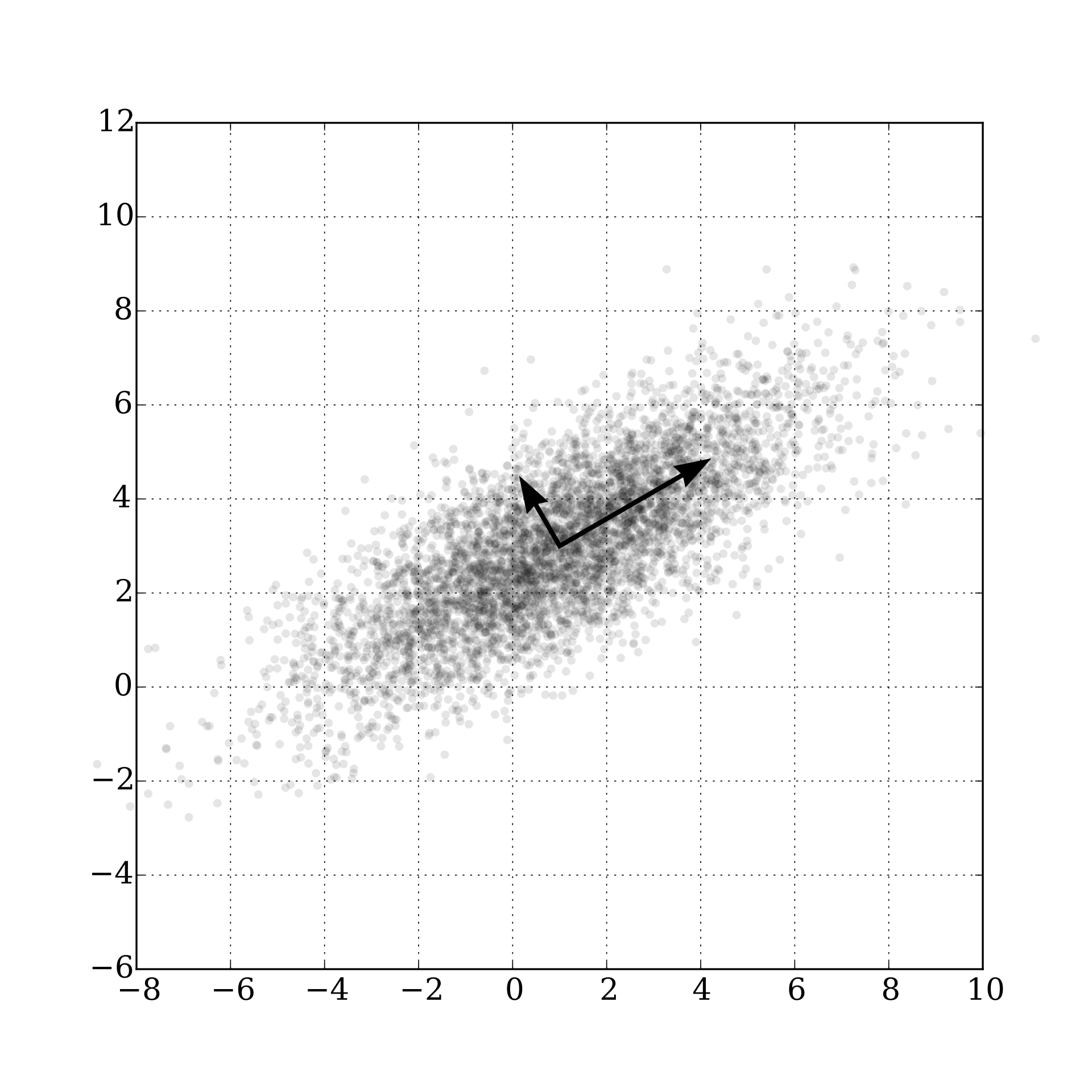
source: wikipedia
We can now discard the least significant dimensions of the final post-PCA data, reducing the number of features in the model. The size of \(F\) dictates the ammount of compression we achieve.
To recover the the original data (or an approximation if \(F\) does not include all features), we invert the transform operation and divide and multiply the transformed data by the inverse of the transformation matrix \(F^{-T}\), i.e.:
Independent Component Analysis
This section was largely inspired on the lecture notes of Tatsuya Yokota, Assistant Professor at Nagoya Institute of Technology
An interesting related topic is the Independent Component Analysis (ICA), a method for Blind Source Separation, a technique that allows one to separate a multidimensional signal into additive subcomponents, under the assumption that:
- the input signals \(s_1\), …, \(s_n\) are statistically independent i.e. \(p(s_1, s_2, ..., s_n) = p(s_1)\,\,p(s_2) \,\, ... \,\, p(s_n)\)
- the values of signals do not follow a Gaussian distributions, otherwise ICA is impossible.
The ICA is based on the Central Limit Theorem that states that the distribution of the sum of \(N\) random variables approaches Gaussian as \(N \rightarrow \infty\). As an example, the throw of a dice has an uniform distribution of 1 to 6, but the distribution of the sum of throws is not uniform — it will be better approximated by a Gaussian as the number of throws increase. Non-Gaussianity is Independence.
A famous example is the cocktail party problem. A guest will be listening to an observed signal \(x\) from an original signal \(s\), as in:
\[\begin{align*} x_1(t) = a_{11}s_1(t) + a_{12}s_2(t) + a_{13}s_3(t)\\ x_2(t) = a_{21}s_1(t) + a_{22}s_2(t) + a_{23}s_3(t)\\ x_3(t) = a_{31}s_1(t) + a_{32}s_2(t) + a_{33}s_3(t) \end{align*}\]We assume that \(s_1\), \(s_2\) and \(s_3\) are statistically independent. The goal of the ICA is to estimate the independent components \(s(t)\) from \(x(t)\), with
\[x(t) = As(t)\]\(A\) is a regular matrix. Thus, we can write the problem as \(s(t) = Bx(t)\), where \(B = A^{-1}\). It is only necessary to estimate \(B\) so that \({ s_i }\) are independent.
White signals are defined as \(z\) such that it satisfies \(E [z] = 0\), and \(E [ z z^T ] = I\). Whitening is useful for the preprocessing of the ICA. The whitening of the signals \(x(t)\) are given by \(z (t) = V x(t)\), where \(V\) is the whitening matrix. Model becomes:
\[s(t) = U z (t) = U V x (t) = B x (t)\]where \(U\) is an orthogonal transform matrix. Whitening simplifies the ICA, so it is only necessary to estimate \(U\). A visual illustration of the source, observerd and whitened data is diplayed below:
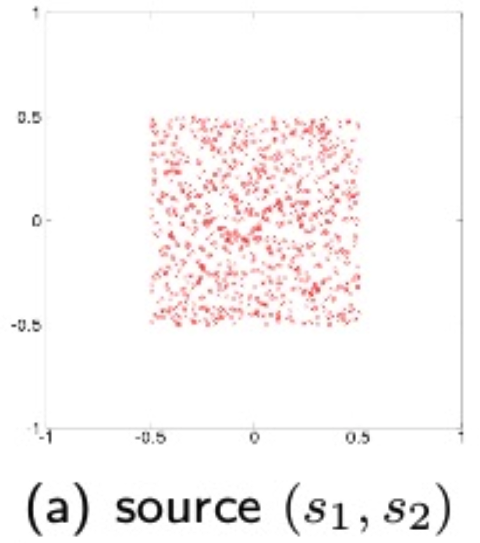
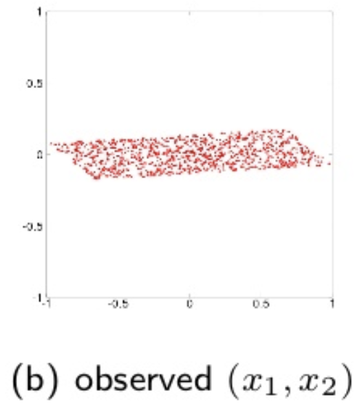
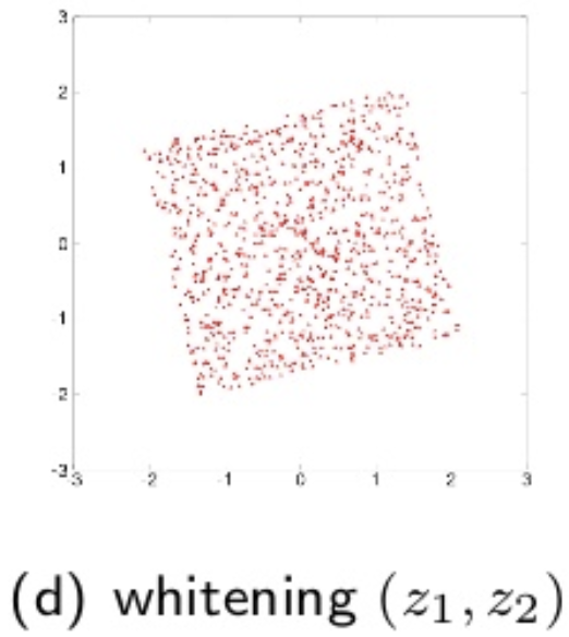
source: T. Yokota, Lecture notes, Nagoya Institute of Technology
** Non-Guassianity is a measure of independence**. Kurtosis is a measure of non-Gaussianity, defined by:
\[k(y) = E [y^4] - 3 (E[y^2])^2.\]We assume that \(y\) is white, i.e. \(E[y]=0\) and \(E[y^2]=1\), thus
\[k(y) = E[y^4]-3.\]We solve the ICA problem with
\[\hat{b} = max_b | k(b^T x(t)) |\]We aim to maximize the absolute value of the kurtosis , i.e. maximize \(\mid k(w^Tz) \mid\) such that \(w^T w=1\). The differential is:
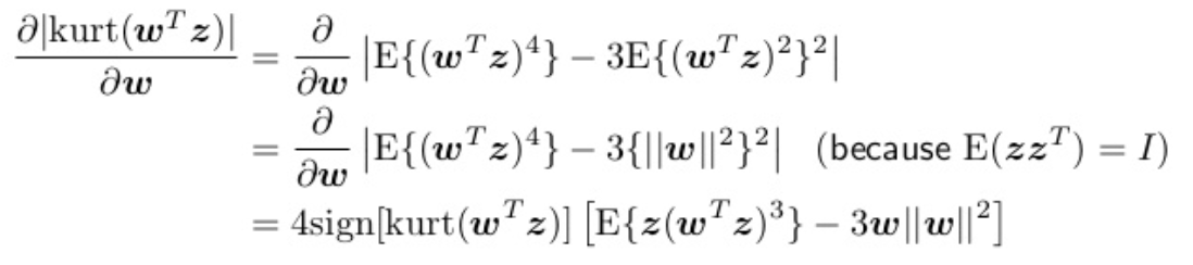
Now we can solve via Gradient descent:
- \(w \leftarrow w + \Delta w\);
- with \(w \propto sign [ k(w^T z)] [ E [ z(w^T z)^3 ] - 3w ]\).
Or… because the algorithm converges when \(w \propto \Delta w\), and \(w\) and \(-w\) are equivalent, by the FastICA as:
- \(w \leftarrow E [ z ( w^T z)^3 ] - 3w\).
As a final remark, it is relevant to mention that kurtosis is very weak with outliers because is a fourth order function. An alternative often used method is the Neg-entropy, robust for outliers. I’ll ommit it for brevity. If you’re interested on details, check the original lecture notes.
Competitive Learning and k-means
Not to be confused with the k-nearest neighbours algorithm (KNN).
Competitive Learning underlies the self organization of the brain. In practice, neural network wiring is adaptive, not fixed. And competition drives wiring across all brain systems (motor cortex, neocortex, etc.). A common technique for data reduction from competitive learning is the prototype clustering, where we represent the datapoints \(x_n\) by a smaller set of prototypes \(w_n\) that represent point clusters. The general rule is that a new point \(x\) belongs to the closest prototype \(k\), i.e.
\[| w_k - x | \leq | w_i - x | \text{, for all } i\]This kind of resolution underlies problems such as the Voronoi diagram for spatial data partitioning. A 2D example follows, where we cluster points in a region (coloured cells) by their prototype (black points):
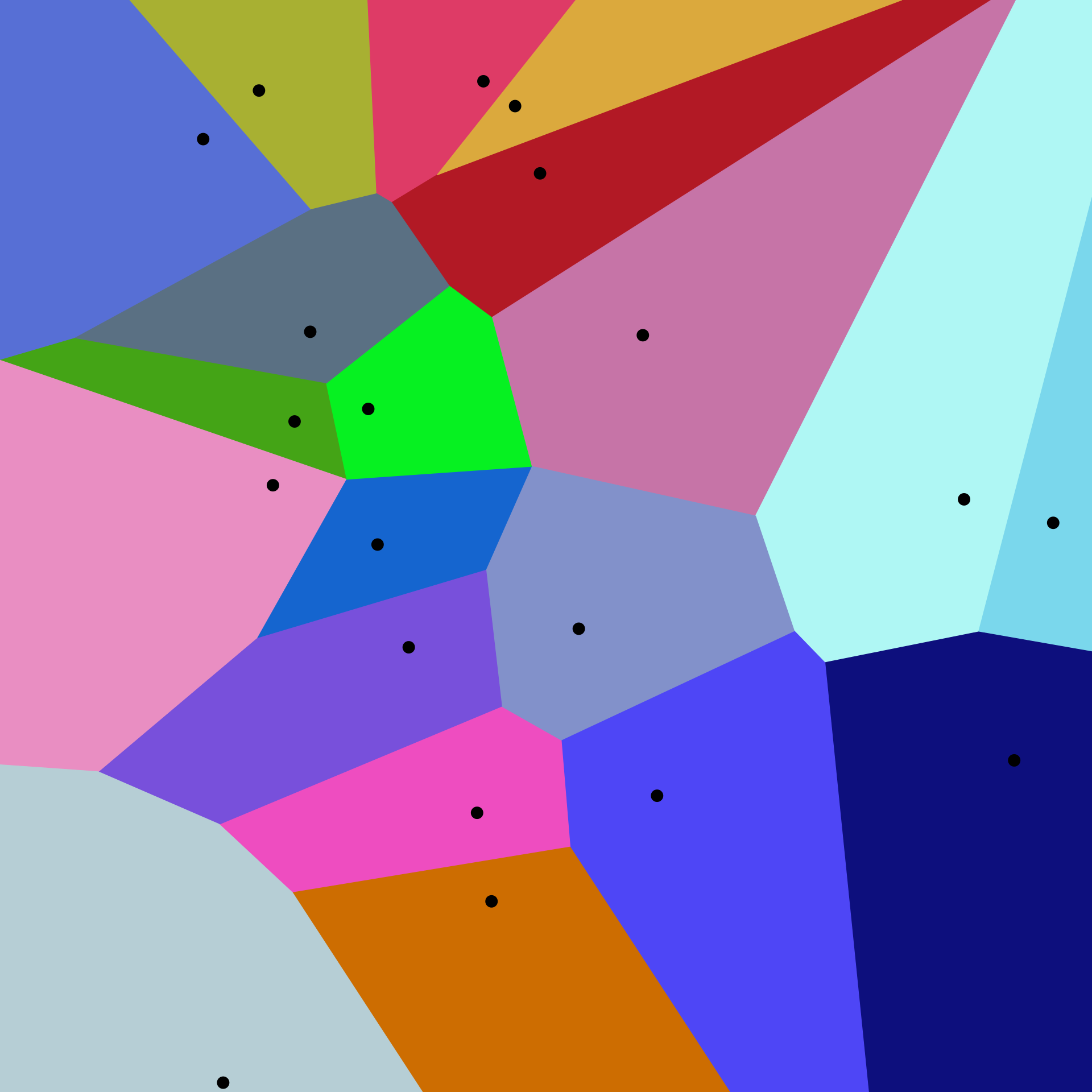
source: wikipedia
Such methods can be applied to e.g. image compression, where one may reduce every RGB pixel in the range \([0-255, 0-255, 0-255]\) to a similar color in a smaller interval or colors. The reconstruction (squared) error is the sum of the error across all datapoints of all clusters \(C\):
\[E = \sum_k \sum_{u \in C_k} (w_k - x_u)^2\]The k-means clustering is an iterative method for propotype clustering. The objective is to find:
\[argmin_s \sum_{i \in [1,k]} \sum_{x \in S_i} || x - w_k ||^2\]The algorithm iteratively performs 2 steps:
- assignment step: assign each observation to the closest mean, based on e.g. Euclidian distance;
- update step: calculate the new means as the centroids of the observations in the new cluster; \(w_i^{(t+1)} = \frac{1}{| C^{(t)}_i |} \sum_{x_j \in C_i^{(t)}} x_j\)
The algorithm converges when the assignements no longer change. This can be shown by the following:
- Convergence means \(\Delta w_i = 0\). So if we have convergence, we must have
which is the definition of center of mass of group \(i\). An illustration of the algorithm follows:
source: wikipedia
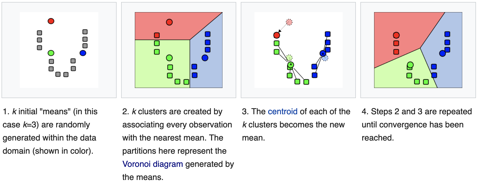
On a 2D universe, one can imagine a 3-cluster algorithm to follow as:
source: wikipedia
The previous update function is a batch learning rule, as it updates the weight based on a set (batch) of inputs. The converse rule is called the online update rule and updates the weights at the introduction of every new input:
\[\Delta w_i = \eta (x_u - w_i)\]which is the Oja’s Hebbian learning rule.
K-means has 2 main problems:
- forces the clusters to be spherical, but sometimes it is desirable to have elliptical clusters;
- each element can only belong to a cluster, but this may not always be a good choice;
Both problems can be fixed with Gaussian Mixture Models. A mixture model corresponds to the mixture of distributions — in this case Gaussians — that represents the probability distribution of observations in the overall population. This content is covered in another post.
Self-Organizing Maps and Kohonen Maps
A self-organizing map (SOM) is an unsupervised artificial neural network, typically applied on a 2D space, that represents a discretization of the input space (or the training set). Its main purpose is to represent training by localized regions (neurons) that represent agglomerates of inputs:
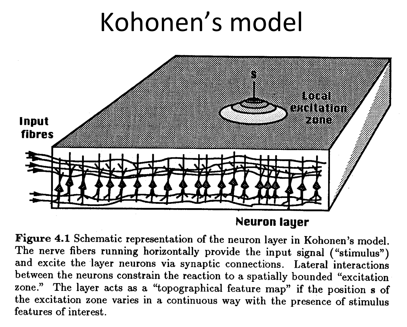
source: Unsupervised and Reinforcement Learning lecture nodes from W. Gerstner at EPFL
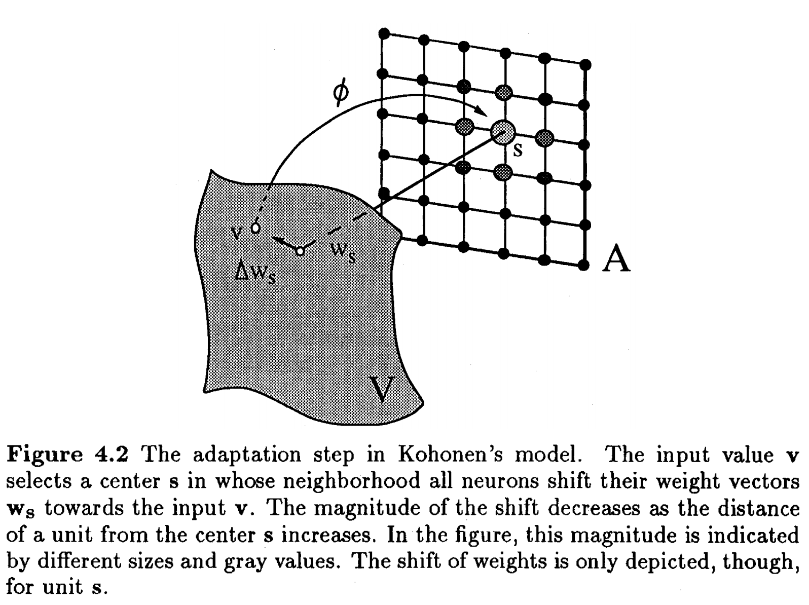
The algorithm is the following:
- neurons are randomly placed in the multidimensional space
- at every iteration, we choose an input \(x_u\);
- We determine which neuron \(k\) is the winner, ie the closest in space:
- Update the weights of the winner and its neighbours, by pulling them closer to the input vector. Here \(\Lambda\) is a restraint due to distance from BMU, usually called the neighborhood function. It is also possible to add \(\alpha(t)\) describing a restraint due to iteration progress.
- repeat until stabilization: either by reaching the maximum iterations count, or difference in weights below a given threshold.
I found a very nice video demonstrating an iterative execution of the Kohonen map in this link and this link.
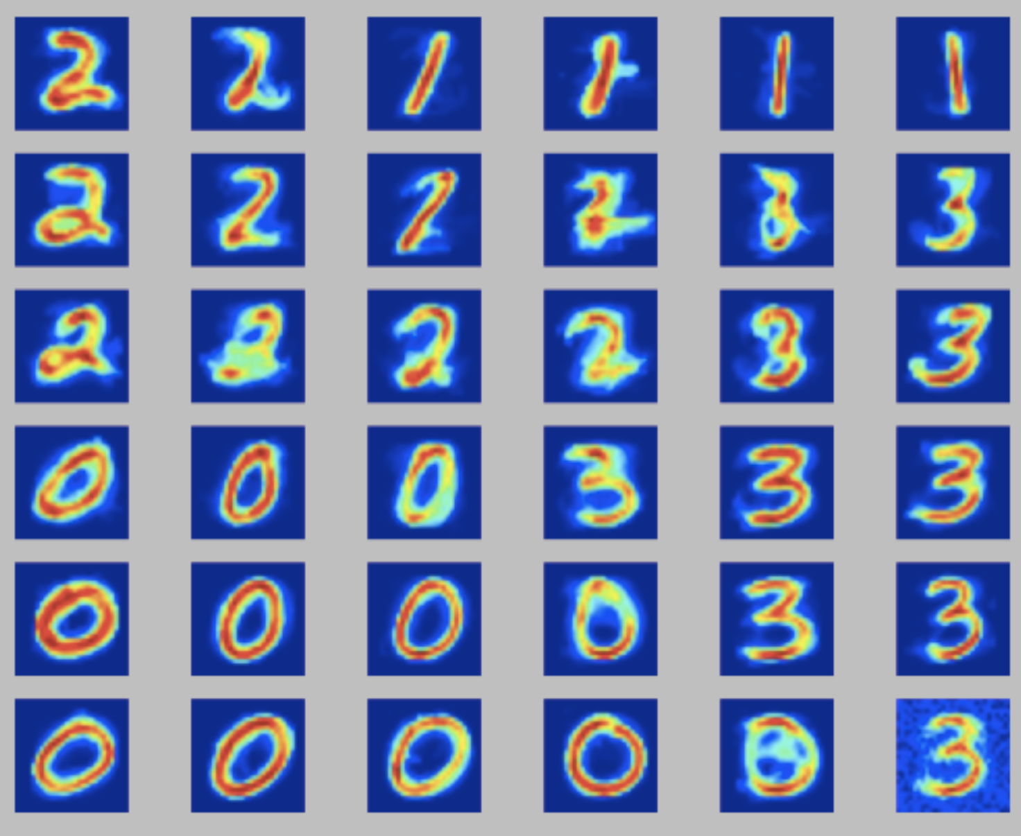
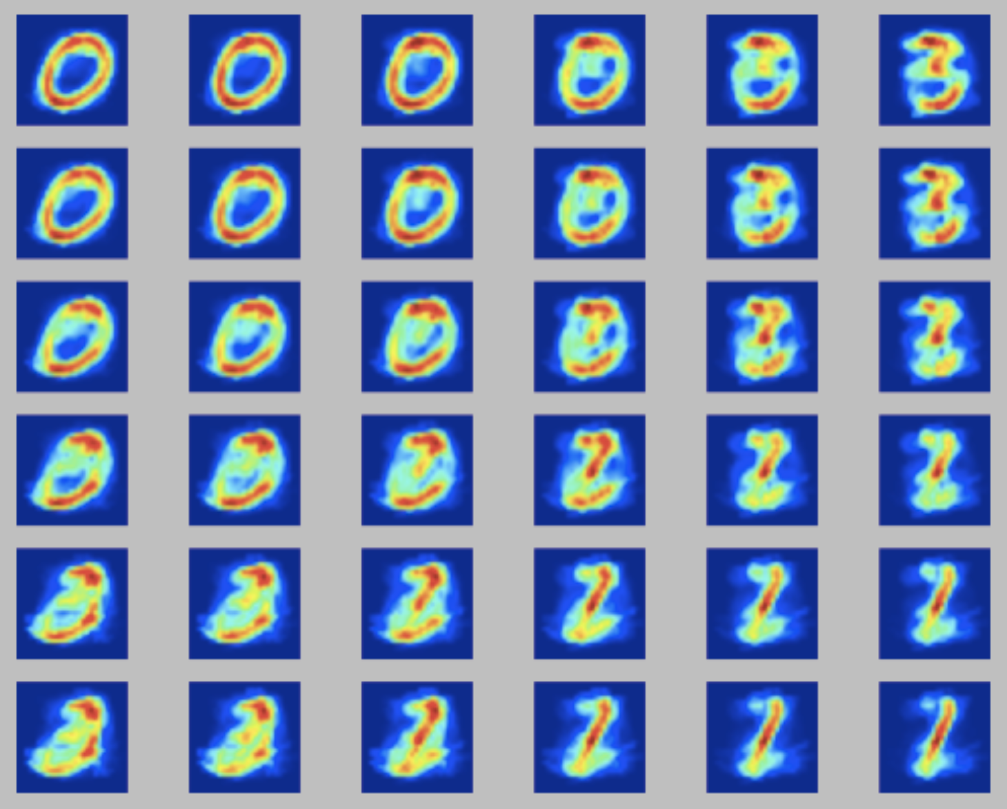
A good example is the detection of hand-written digits on a trained dataset of the MNIST database. For simplicity, we will work only with digits from 0 to 9. Each digit is a 28x28 (=784) pixel array, represented as data point on a 784-d dataspace. Each pixels is monochromatic, thus each dimension is limited to values between 0 and 256. Our task is to, given a database of 5000 handwritten digits, find the best 6x6 SOM that best represents 4 numbers from 0-9. We will study how choosing the right neighborhood width and learning rate affect the performance of the Kohonen map.
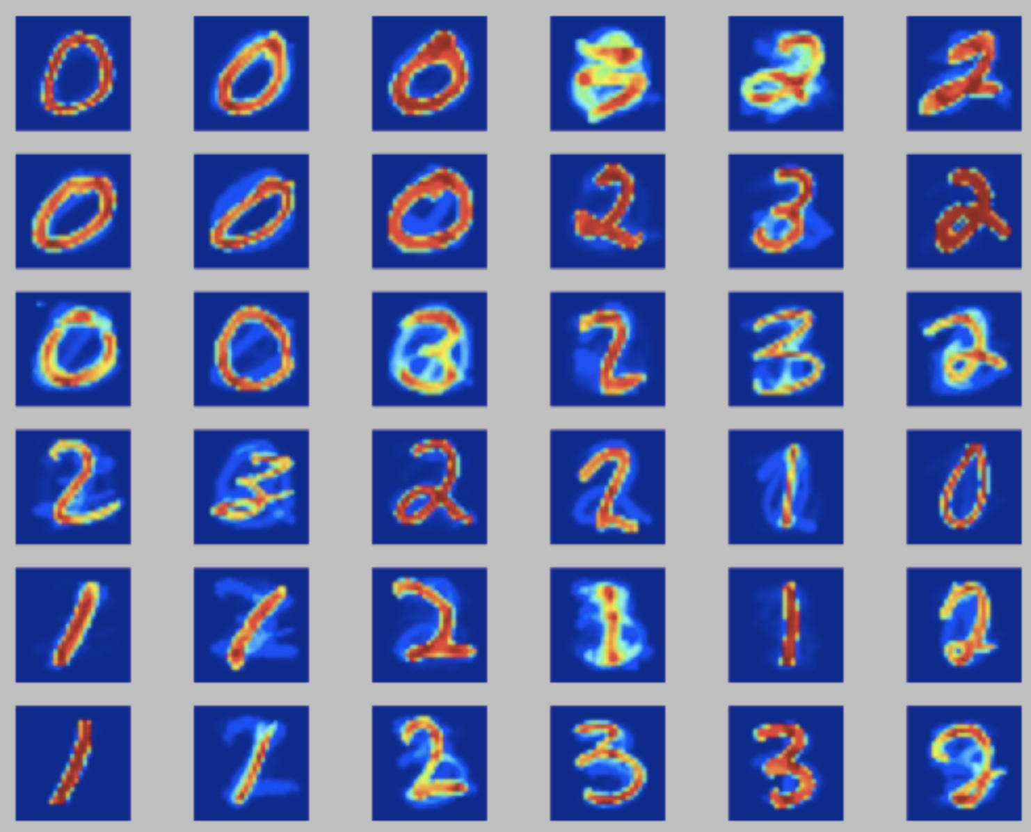
The input dataset and the python implementation are available in kohonen_mnist.zip. The goal is to fine-tune the neighboring and learning rate \(\eta\) parameters. A good solution would give you some visual perception of the numbers being identified (in this case 0, 1, 2 and 3). Here I discuss three possible outputs:
- left: a nicely tuned SOM, where each quadrant of neurons represents a digit;
- center: a SOM with a high learning rate. The large step size makes neurons step for too long distances during trainig, leading to a mixing of digits on proximal neurons and possibly a tangled SOM web;
- right: a SOM with a high neighborhood width. The high width causes all neurons to behave almost synchronously, due tot he very wide range of the udpate function. This leads to very similar outputs per neuron;
For more examples, check the wikipedia entry for Self Organizing maps.
The Curse of Dimensionality
As a final remark, distance-based methods struggle with high dimensionality data. This is particularly relevant on Euclidian distances. This is due to a phenomen denominated the Curse of Dimensionality that states that the distance between any two given elements in a multidimensional space becomes similar as we increase the number of dimensions, deeming the distance metric almost irrelevant. I will not detail the soundness of the claim, but check this blog post if you are interested in knowing the details.