Distributed GPT model (part 3): model parallelism with Megatron-LM
This post follows from the previous posts Distributed training of a GPT model using DeepSpeed and Distributed training of a GPT model using DeepSpeed, where we implemented Data and Pipeline parallelism on a GPT model. Data and pipeline parallelism are 2 dimensions of the 3D parallelism of ML models, via Data, Pipeline and Tensors/Models parallelism. In this post, we will discuss model (tensor) parallelism, particularly the Megatron-LM implementation.
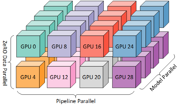
The 3D parallelism aims and partitioning (color-coded) computer resources across the 3D space of data, pipeline and tensor (model) dimensions. In this post of will focus on model/tensor parallelism. Source: Microsoft Research Blog
Tensor parallelism, vertical parallelism, intra-layer parallelism, activation parallelism or most commonly ad confusedly called model parallelism, is the third dimension of parallelism and aims at partitioning the computation on the activations dimension. This is a hard problem: in practice we must decide for the dimension of tensor partitioning (row, wise, none) and adapt the communication and computation accordingly. Therefore, it is a model- and data-specific implementation.

A representation of tensor parallelism on a fully-connected DNN, on two processors \(p0\) and \(p1\). Input sample and activations are distributed across different processors. Red lines represents the activations that have to be communicated to a different processor.
Looking at the previous picture, we notice a major drawback in this method. During training, processors need to continuously communicate activations that are needed across the processor network. This communication is synchronous and does not allow an overlap with compute. And it creates a major drawback on the execution as it requires a tremendous ammount of communication at every layer of the network and for every input batch.
There are several alternative ways to distribute multi-dimensional tensors across several compute nodes, that aim at reducing number of comunication steps or ammount of communcation volue. In this post, we will detail and implement Megatron-LM paper.
Megatron-LM model parallelism
We can have a better understanding if we try to replicate the partitioning suggested by Megatron-LM in the paper Megatron-LM: Training Multi-Billion Parameter Language Models Using Model Parallelism. The main rationale in Megatron-LM is that Transformer-based models have two main components - a feed-forward (MLP) and an attention head - and we can do a forward and a backward pass on each of these blocks with a single collective communication step.
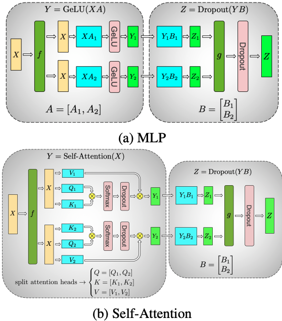
The MLP and self-attention blocks in the Megatron-LM implementation. f and g are conjugate identity and all-reduce operations that c. f is an identity operator in the forward pass and all reduce in the backward pass while g is an all reduce in the forward pass and identity in the backward pass. Source: Megatron-LM paper
The rationale is the following: the MLP is sequence of (1) a MatMul \(AX\), (2) a ReLU \(Y\); a (3) MatMul \(YB\) and a (4) dropout layer. Let’s focus on the first two operations:
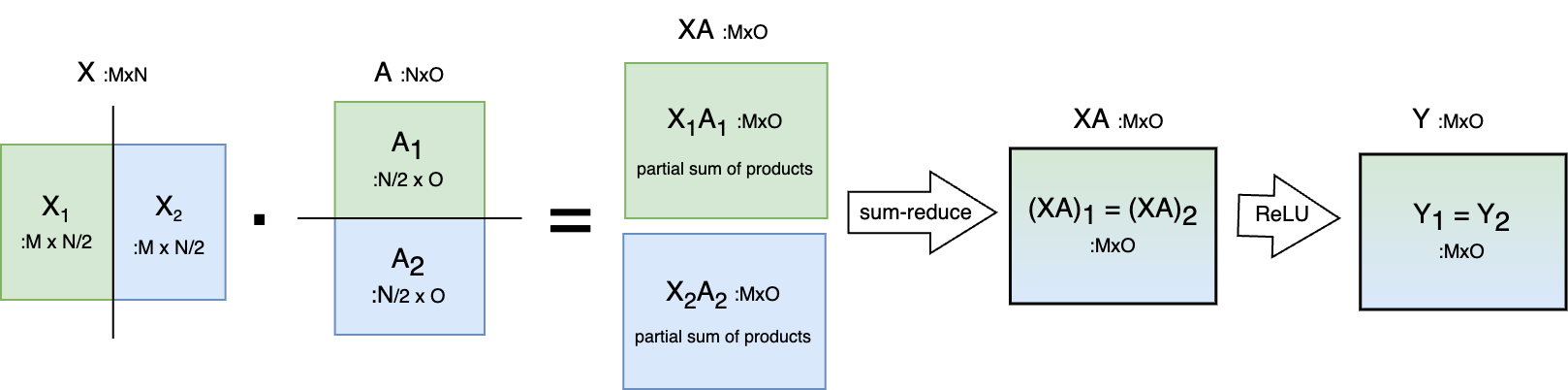
- “One option to parallelize the GEMM is to split the weight matrix \(A\) along its rows and input \(X\) along its columns. […] This partitioning will result in \(Y = GeLU(X_1 A_1 + X_2 A_2)\). Since GeLU is a nonlinear function, \(GeLU (X_1 A_1 + X_2 A_ 2) \neq GeLU( X_1 A_1 ) + GeLU (X_2 A_2)\) and this approach will require a synchronization point (sum-reduce) before the GeLU function”. We can follow this approach - pictured below - for each of the 2 MatMuls, yielding a total of two communication steps.
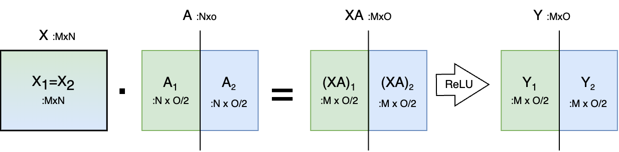
- Another option is to don’t split \(X\) and split \(A\) along its columns, that “allows the GeLU nonlinearity to be independently applied to the output of each partitioned GEMM”. The output of the ReLU \(Y\) is then \([Y_1, Y_2] = [GeLU (X A_1), GeLU(X A_2)]\) and this removes a synchrnization point. After the MatMul and ReLU is done, we must follow with another MatMul and a dropout. Note that if we follow this approach (pictured below), the output \(Y\) of the first MatMul (which is the input for the second MatMul) is split column-wise. Therefore, Megatron will then use the previous approach for the second MatMul, that requires 1 collective communication step. We therefore perform 1 communication step for 2 MatMuls.
The algorithm of the attention mechanism is analogous, except that instead of a single MatMul \(AX\) at the beginning of the workflow, we perform three MatMuls \(XV\), \(XQ\) and \(XK\) for the value, query and key matrices of the attention mechanism. Therefore, this algorithm requires one (not two) communication steps per MLP and attention block.
Megatron-LM makes this implementation very simple, by adding only the \(f\) and \(g\) functions to the serial use case. Following the paper: “\(f\) is an identity operator in the forward pass and all reduce in the backward pass while \(g\) is an all reduce in the forward pass and identity in the backward pass”. So we can implement this as:
class Megatron_f(torch.autograd.Function):
  """ The f function in Figure 3 in Megratron paper """

  @staticmethod
  def forward(ctx, x, mp_comm_group=None):
      ctx.mp_comm_group = mp_comm_group #save for backward pass
      return x

  @staticmethod
  def backward(ctx, gradient):
      dist.all_reduce(gradient, dist.ReduceOp.SUM, group=ctx.mp_comm_group)
      return gradient
and
class Megatron_g(torch.autograd.Function):
  """ The g function in Figure 3 in Megratron paper """

  @staticmethod
  def forward(ctx, x, mp_comm_group=None):
      dist.all_reduce(x, dist.ReduceOp.SUM, group=mp_comm_group)
      return x

  @staticmethod
  def backward(ctx, gradient):
      return gradient
Note that we added an extra argument mp_comm_group that refers to the model-parallel communication group. This refers to the communication group is to allow us to combine MP with other types of parallelism. As an example, if you have 8 GPUs, you can have 2 data parallel groups of 4 model parallel GPUs. We now add model parallelism to the MLP by inserting \(f\) and \(g\) in the forward pass, at the beginning and end of the block, just like in the paper:
class Megatron_FeedForward(nn.Module):
  """ the feed forward network (FFN), with tensor parallelism as in Megatron-LM MLP block"""

  def __init__(self, n_embd, mp_comm_group=None):
    super().__init__()
    self.mp_comm_group = mp_comm_group

    #Fig 3a. MLP: splits first GEMM across colums and second GEMM across rows
    n_embd_mid = n_embd*4 #width of MLP middle layer, as before
    if self.mp_comm_group:
        n_embd_mid //= dist.get_world_size()

    self.fc1 = nn.Linear(n_embd, n_embd_mid)
    self.fc2 = nn.Linear(n_embd_mid, n_embd)
    self.dropout = nn.Dropout(dropout)

  def forward(self, x):
    if self.mp_comm_group:
        x = Megatron_f.apply(x, self.mp_comm_group) #Fig 3a. apply f on input

    y = F.relu(self.fc1(x))
    z = self.fc2(y)

    if self.mp_comm_group:
        z = Megatron_g.apply(z, self.mp_comm_group) #Fig 3a. apply g before dropout

    z = self.dropout(z)
    return z
The attention head follows a similar approach, where we apply the tensor reduction to all the key, query and value tensors:
class Megatron_Head(nn.Module):
  """ the attention block with tensor parallelism as in Megatron-LM paper"""

  def __init__(self, head_size, mp_comm_group=None):
    super().__init__()

    self.mp_comm_group = mp_comm_group
    if mp_comm_group:
        #Fig 3b. Self-attention: splits first GEMM across colums and second GEMM across rows
        head_size //= dist.get_world_size()

    self.key   = nn.Linear(n_embd, head_size, bias=False)
    self.query = nn.Linear(n_embd, head_size, bias=False)
    self.value = nn.Linear(n_embd, head_size, bias=False)
    self.register_buffer('tril', torch.tril(torch.ones(block_size, block_size)))
    self.dropout = nn.Dropout(dropout)

  def forward(self, x):
    B,T,C = x.shape

    if self.mp_comm_group:
      x = Megatron_f.apply(x, self.mp_comm_group) #Fig 3b. apply f on input

    k = self.key(x) #shape (B,T, head_size)
    q = self.query(x) #shape (B,T, head_size)
    v = self.value(x) #shape (B,T, head_size)

    # compute self-attention scores
    # [...] as before

    if self.mp_comm_group:
      wei = Megatron_g.apply(wei, self.mp_comm_group) #Fig 3b. apply g after dropout

    #perform weighted aggregation of values
    out = wei @ v # (B, T, T) @ (B, T, head_size) --> (B, T, head_size)
    return out
Detour: model parallelism on Convolutional Neural Nets
The whole point of Megatron-LM was to reduce the ammount of high volume communication steps due to the high volume of data involved per step. However, it is relevant to mention that model parallelism has some use cases where it can be efficient and of low volume communication. An example is on the parallelism of Convolutional Neural Networks. In practice, due to the kernel operator in CNNs (that has a short spatial span), the amount of activations to be communicated is limited to the ones ones that neighboring activations need. This method has been detailed by Dryden et al. (Improving Strong-Scaling of CNN Training by Exploiting Finer-Grained Parallelism, Proc. IPDPS 2019). The functioning is illustrated in the picture below and is as follows:
- Input data and activations are split across the height and width dimensions among processors;
- For a given convolutional layer, the convolution can be computed in independently be each processor, with the exception of the activation in the split boundaries. These activations (the halo region in purple in the picture blow) will need to be communicated at every forward/step.
Illustration of model parallelism applied to Convolutional Neural network. LEFT: splitting of activations on a 2D input across four processors \(p0-p3\). red box: center of the 3x3 convolution filter; red arrow: data movement required for updating neuron in center of filter; violet region: halo region formed of the elements that need to be communicated at every step. RIGHT: communication between processors \(p0\) and \(p1\). Red arrow: forward pass dependencies; blue arrow: backward pass dependencies;
Final remarks and code
There is ongoing work from PyTorch to support general model parallelism, where the user can pick row-wise split, column-wise split and sharding of individual tensor. Also, combining data, pipeline and model parallelism requires one to define the corect strategy for custom model parallelism.
As an important remark: finding the best parallelism strategy is hard, due to the high number of hyper-paramemers: ZeRO stages, offloading, activation checkpointing intervals, pipeline parallelism stages, data parallelism, model parallelism, etc, as it depends on the ML model, data and hardware. In practice, our config file and parallelism settings are a manually-optimized ballpark figure of the default config file with some parameter grid search. In this topic, there is still plenty of work to be done to make it optimal, possibly by exploring the autotuning tools in DeepSpeed.
We just scratched the surface of DeepSpeed capabilities. There are plenty of resources that should also be explored. To name a few: autotuning (README.md) for parallelism hyper-parameters discovery; flops profiler measures the time, flops and parameters of individual layers, sparse attention kernels (API) to support long sequences of model inputs, such as text, image, or sound; communication optimizers offer the same convergence as Adam/LAMB but incur 26x less communication and 6.6x higher throughput on large BERT pretraining, monitor to log live training metrics to TensorBoard, csv file or other backend; model compression (API) via layer reduction, weight quantization, activation quantization, sparse pruning, row pruning, head pruning and channel pruning, to deliver faster speed and smaller model size.
Finally, the Megatron-LM model parallelism code has been added to the GPT-lite-distributed repo, if you want to try it.