Distributed GPT model: data parallelism, sharding and CPU offloading
Distributed data parallelism (DDP) refers to the parallel execution of different input samples across processors. If you consider any data input to be of shape \(B \times T \times E\) as in batch size, sequence/temporal size, and embedding/features size, then data parallelism refers to the use case where we split the data across \(P\) processes, leading to a local input of shape \(B/P \times T \times E\):
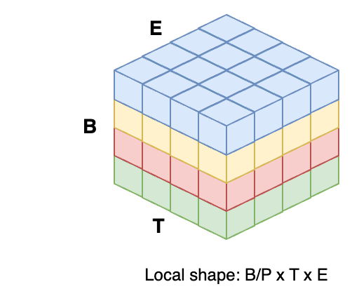
An illustration of the DDP data layout, split across 4 processes colorcoded as blue, yellow, red and green.
In this post, we will perform distributed data parallelism on the training process of the GPT-lite model we built in the previous post, on a network of 8 GPUs, using PyTorch’s PyTorch and DeepSpeed ZeRO (Zero Redundancy Optimizer, a lightweight wrapper on PyTorch).
There are two main data parallelism approaches:
Distributed Data Parallelism keeps a full copy of the model (weights, optimizer parameters and gradients) on each processor. All models are initialized equally. Each processor takes as input a different minibatch and performs a forward pass to compute the loss that relates to that batch. On the backward pass, at every layer of the model, all processes compute the gradients of that batch, and perform an all-reduce to get the mean gradients across all processors. This is then used to update the optimizer states. Because parameters are initialized equally, and the gradients are mean-reduced, and all parameters perform the same updates, the models across all processors are kept in an identical state throughout the execution.
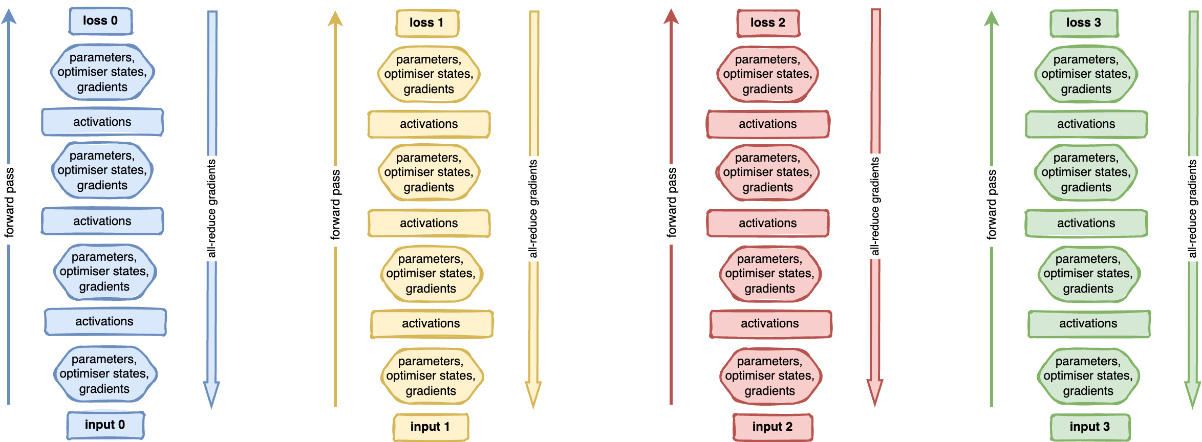
Workflow for distributed data parallelism (DDP) across 4 color-coded processes. Each process holds a copy of a 4-layer feed-forward model, initialized identically. Each process performs a forward pass of its own data (arrow pointing up on the left of the model). On the backward pass, all processes compute the local gradients and mean-reduce them across the network (arrow pointing down on the right of the model). The mean of the gradients is then used by the optimizer to update the parameter states.
Looking at the previous, we can see that each processor holds a copy of the model and this leads to a superfluos memory usage. That’s where sharding comes into play.
(Fully-)Sharded Data Parallelism (FSDP) a.k.a sharding is a distributed setup where processors dont hold a full copy of the model, but only the parameters, optimizer states and gradients of a subset of layers. As before, different processors input different mini-batches. In DeepSpeed lingo, sharding goes by the name of ZeRO (Zero Redundancy Optimizer). ZeRO has several alternative execution modes (stages). Each stage represents a different level of memory redundancy, corresponding to different variable types being distributed or replicated across nodes:
- ZeRO stage 0: no sharding of any variables, being equivalent to Distributed Data Parallelism;
- ZeRO stage 1 (ZeRO-1): the optimizer states (e.g., for Adam optimizer, the weights, and the first and second moment estimates) are partitioned across the processes. Affects only the backward pass.
- ZeRO stage 2 (ZeRO-2): the gradients for updating the model weights are also partitioned such that each process retains only the gradients corresponding to its portion of the optimizer states. Also relevant only for the backward pass.
- ZeRO stage 3 (ZeRO-3): the model parameters are partitioned across the processes. Includes a communication overhead on both the forward and backward passes.
An important remark is that activations are not sharded i.e. they are kept in full shape on each processor. And in modern models, a huge chunk of memory is allocated to residual memory (activations, normalization layers, etc) which is not sharded by FSDP. With that in mind, the following diagram illustrates the workflow of the stage 3 sharding (of parameters, gradients and optimizer states):
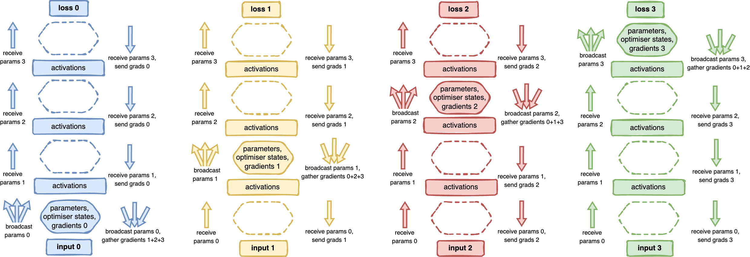
Workflow for stage 3 sharding. Each processor contains a non-overlapping subset of parameters, gradients and optimiser data, split by assigning different layers to different processes. Each processor loads a different data batch. During forward and backward passes (represented by arrows on the left and right of model, respectively), when computing is needed for a given layer, the process who is responsible for those layers will broadcasts and gather those values to/from the remaining processes. Example for processor 1 (yellow): Data loading: yellow process loads data sample 1. Forward pass: yellow process receives the parameters from rank 0 (blue) and computes the activations for layer 1. Afterwards, yellow process broadcasts its parameters to ranks 0, 2 and 3, so that they compute their activations for layer 2. Activations for layer 3 and 4 are computed similarly to layer 1, led by the red and green processes, specifically. Backward pass: the green process (3) broadcasts parameters to all other processes. Each process can use its activations and the received parameters to compute the gradients for the top layer. All processes gather their local gradients in process 3 that will use it to update the parameters of the last layer. For the remaining layers, the same happens, where the red, yellow and blue processes will be the ones doing the broadcast of parameters and gather of gradients (iteratively).
The higher the stage, the more communication we require, but the less memory we consume. These memory improvements are summarized in the Microsoft Research blog as:
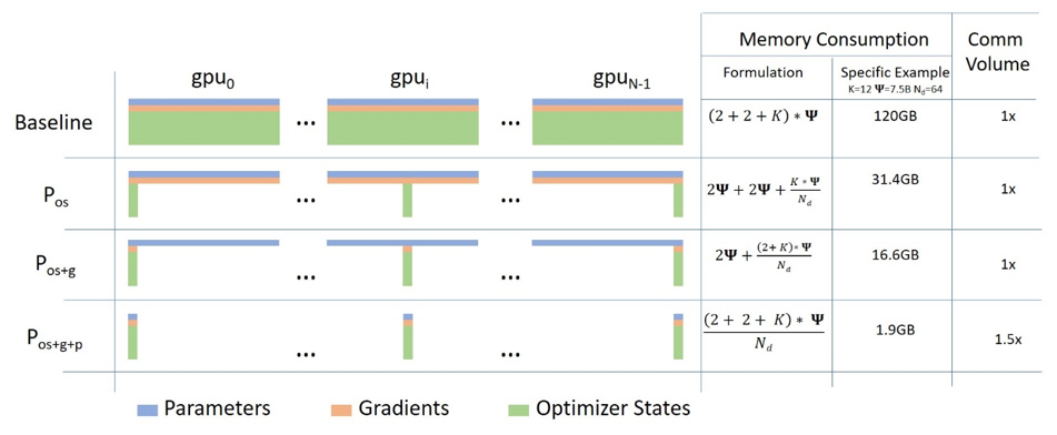
Memory consumption of the three different stages of ZeRO FSDP. Source: Microsoft Research blog
CPU Offloading
Sometimes the model can be so big that even with sharding, it won’t fit in a single process. A common technique to handle such memory limitations is CPU offloading - also referred to as virtual Deep Neural Networks by vDNN (Rhu et al.) and vDNN+ (Shiram et al). The main goal of this method is to iteratively move to the GPU the portions of activations and model that are required for the current and following subset of computation steps. Previously-processed layers are moved from GPU to CPU while upcoming layers will be moved from the CPU to GPU.
This is possible because as we’ve seen on a previous post, the loss (and its derivative) can be written as a composition of activations throughout layers, e.g. for MAE:
\[L = \frac{1}{N} \sum_{n=1}^N | y_n - f^{(L+1)} \circ ... \circ f^{(2)} \circ f^{(1)} (x_n^{(0)}) |\]where \(f^{(l)}\) is the activation function in layer \(l\) and \(y\) is the groundtruth. The important concept here is the composition of the \(f\) function throughout layers. To reduce the waiting time on pushing (pulling) a layer to (from) the GPU, we can overlap computation of current layers with communication of upcoming ones. The forward pass can be illustrated as:

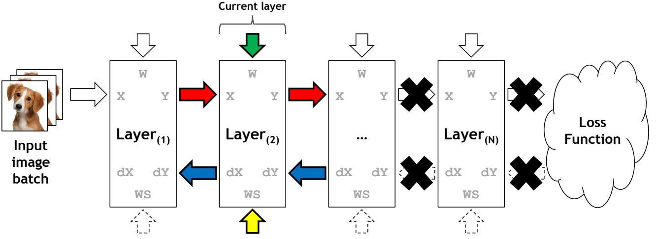
The forward pass on the vDNN(+) implementation on convolutional neural networks. Red arrays represent the data flow of variables \(x\) and \(y\) (layers input and output) during forward propagation. Green arrows represent weight variables. Yellow arrows represent the variables workspace in cuDNN, needed in certain convolutional algorithms. Data not associated with the current layer being processed (layer N) is marked with a black cross and can safely be removed from the GPU’s memory. Source: vDNN (Rhu et al.)
The backward propagation phase is trickier, as it also includes the gradients being propagated down the model:
The back propagation phase on the vDNN(+) implementation on convolutional neural networks. Red arrays represent the data flow of variables \(x\) and \(y\) (layers input and output) during forward propagation. Blue arrows represent data flow during backward progagation. Green arrows represent weight variables. Yellow arrows represent the variables workspace in cuDNN, needed in certain convolutional algorithms. Data not associated with the current layer being processed (layer 2) is marked with a black cross and can safely be removed from the GPU’s memory. Source: vDNN (Rhu et al.)
Model and dataset setup
We start our implementation by taking our previous GPT-lite with the specs matching the GPT-2 Small model in Language Models are Few-Shot Learners (Fig 2.1):
n_layer = 12   # depth of the network as number of decoder blocks.
n_embd = 768   # size of the embeddings (d_model)
n_head = 12   # number of attention heads in the Multi-Attention mechanism
block_size = 2048   # block size ie max number of training sequence, the $n_{ctx}$ in the paper .
dropout = 0.1   # dropout rate (variable p) for dropout units
We then define the methods get_model() and get_dataset() that return our model and the tiny shakespeare dataset:
## gptlite.py

def get_dataset():

  class GPTliteDataset(torch.utils.data.Dataset):

      def __init__(self, train_data, block_size):
        self.train_data = train_data
        self.block_size = block_size

      def __len__(self):
        return len(self.train_data)

      def __getitem__(self, idx):
        # generate 1 random offset on the data
        ix = torch.randint(len(self.train_data)-self.block_size , size=())
        # input is a random subset of tokens
        x = self.train_data[ix   : ix+self.block_size]
        # target is just x shifted right (ie the next predicted word)
        y = self.train_data[ix+1 : ix+1+self.block_size]
        return x, y

  train_data, valid_dataset, vocab_size = load_tiny_shakespeare_data()
  train_dataset = GPTliteDataset(train_data, gptlite.block_size)
  valid_dataset = GPTliteDataset(valid_data, gptlite.block_size)
  return train_dataset, valid_dataset, vocab_size


def get_model(vocab_size):
  return GPTlite(vocab_size)
Detour: using a pre-existing model
Note that code this code is applicable to any model of type torch.nn.Module and any dataset of type torch.utils.data.Dataset. As an example. if you wanted to perform a multi-class classification using the ResNet network on the CIFAR10 dataset available in torchvision, you could define the previous 2 methods as:
import torchvision

def get_dataset():
  import torchvision.transforms as transforms
  transform = transforms.Compose([
    transforms.ToTensor(),
    transforms.Normalize((0.5, 0.5, 0.5), (0.5, 0.5, 0.5))
  ])
  dataset = torchvision.datasets.CIFAR10(
    root='./data', train=True, download=True, transform=transform)
  return dataset

def get_model(num_classes):
  return torchvision.models.resnet18(num_classes=num_classes)
PyTorch implementation
We will now impement data parallelism in PyTorch. Firstly, we collect the global variables that are set by the torchrun launcher (detailed below), as they’re important to uniquely identify processes in the network and GPU devices within a node:
import os
rank = int(os.environ['RANK'])   # the unique id across all processes in all nodes
local_rank = int(os.environ['LOCAL_RANK'])   # the unique id across this node
world_size = int(os.environ['WORLD_SIZE'])   # the number of processes across all nodes
Now we define the DataLoader that tells each process how to iterate through the data:
dataloader = torch.utils.data.DataLoader(dataset, batch_size=4, sampler=sampler)
Note the argument sampler, that is a DistributedSampler that will delegate different samples from the dataloader to different processes. Without this, all processes would load exactly the same datapoints in every iteration.
sampler = torch.utils.data.distributed.DistributedSampler(
  dataset, num_replicas=world_size, rank=rank)
We then place each model in a different GPU with the correct data type:
device = f"cuda:{local_rank}"
dtype = torch.bfloat16
model = model.to(device=device, dtype=dtype)
and we finally wrap it with the DistributedDataParallel for the DDP implementation:
model = torch.nn.parallel.DistributedDataParallel(model, device_ids=[device])
or with the FullyShardedDataParallel wrapper for the sharded implemetation, as:
model = torch.distributed.fsdp.FullyShardedDataParallel(
    model,
    device_id=self.device,
    sharding_strategy=torch.distributed.fsdp.api.ShardingStrategy.SHARD_GRAD_OP, # define the stage here
)
And that’s it. Now you can write your training loop normally and torch will do all the communication and synchronization under the hood:
for step, data in enumerate(dataloader):
  inputs = data[0].to(engine.device)
  labels = data[1].to(engine.device)
  outputs = engine(inputs)  # fwd pass
  loss = torch.nn.functional.cross_entropy(outputs, labels) # loss
  loss.backward() # compute gradients
  optimizer.step() # update parameters
  optimizer.zero_grad(set_to_none=True)
Because gradients are computed and mean-reduced from the top to the bottom layer of the model, we can overlap the computation of the gradients from the lower layers with communication of the upper layers, as we go along our backward pass. According to the PyTorch DDP documentation:
The backward pass iteratively computes gradients (from last to first layer) and collects blocks of gradients to be communicated. These blocks will be mean-reduced asynchronously during the backward pass, while the computation for the backward pass proceeds. Therefore it overlaps backward pass computation with gradients communication. At the end of the backward pass, all GPUs wait for all gradient all-reduces to finish, and then triggers the parameter updates.
For extra memory savings, offloading of tensors can also be achieved via PyTorch by using custom hooks for autograd saved tensors.
Finally, you can launch the application by calling torchrun. Torchrun is a network bootstrapper that spaws a python script across compute all compute nodes in a network and sets the previous environmental variables that allow for processes to be uniquely identifiable across the network. The usage is simple:
$ torch --standalone, --nproc_per_node=4, ./train.py
where nproc_per_node is the number of GPUs on each node.
DeepSpeed implementation
Implementing an existing code in DeepSpeed is pretty simple. To start, DeepSpeed features can be activated via the deepspeed API or its Configuration JSON. The number of possible optimizations is large, as it can defines parallelism, floating point precision, logger, communication parameters, etc. In our implementation, we will start with a simple config file, where we configure the DeepSpeed logger to output memory and throughput info at every 10 epochs (steps_per_print), we set the batch size to 256 and (optionally) define the settings of the optimizer (optimizer) and learning rate scheduler (scheduler):
{
  "train_batch_size": 256,
  "steps_per_print": 10,
  "optimizer": {
    "type": "AdamW",
    "params": { "lr": 0.001, "betas": [ 0.8, 0.999  ], "eps": 1e-8, "weight_decay": 3e-7 }
  },
  "scheduler": {
    "type": "WarmupLR",
    "params": { "warmup_min_lr": 0, "warmup_max_lr": 0.001, "warmup_num_steps": 1000 }
  }
}
Note that in DeepSpeed lingo, the train_micro_batch_size_per_gpu refers to the batch size loaded per dataloader (ie per node, per gradient accumulation step), while train_batch_size refers to the batch size across all gradient accumulation steps and processes in the network ie:
train_batch_size = train_micro_batch_size_per_gpu * num_gpus * num_nodes * gradient_accumulation_steps
Therefore, Gradient accumulation can be enable by simply setting train_micro_batch_size_per_gpu.
ZeRO Fully-Sharded Data Parallelism can be activated by specifying the relevant stage in the config file. If omitted, or when passing the stage 0, DeepSpeed is disabled and the execution follows a regular distributed data paralllel workflow:
{
  "zero_optimization": { "stage": 3 }
}
CPU offloading on DeepSpeed is called ZeRO-Offload, as a system for offloading optimizer and gradient states to CPU memory. On top of stage 3, we can enable ZeRO-Infinity, also an offloading engine that extends ZeRO-offload with support to NVMe memory. According to the ZeRO-3 documentation, “ZeRO-Infinity has all of the savings of ZeRO-Offload, plus is able to offload more the model weights and has more effective bandwidth utilization and overlapping of computation and communication”. They can be enabled via:
{
  "zero_optimization": {
    "stage": 3,
    "offload_optimizer": { "device": "cpu", "pin_memory": true },
    "offload_param": { "device": "cpu", "pin_memory": true },
  }
}
We’re almost done now. Once we have our config file properly calibrated, the implementation is straighforward. All boilerplate that PyTorch requires for parallelism and data loaders is managed internally by DeepSpeed. So we only need to setup DeepSpeed as:
def main_deepspeed(n_epochs=100, random_seed=42):

  torch.manual_seed(random_seed)  #set random seed (used by DataLoader)
  deepspeed.runtime.utils.set_random_seed(random_seed) #set DeepSpeed seed
  deepspeed.init_distributed()  # initialize distributed DeepSpeed
  config = 'ds_config.json'  # load the DeepSpeed config
  criterion = torch.nn.CrossEntropyLoss()  # initialize loss function
  train_dataset, _, vocab_size = gptlite.get_dataset()  # initialize GPT-lite dataset
  model = gptlite.get_model(vocab_size)  # initialize GPT-lite model

  engine, optimizer, train_dataloader , _ = deepspeed.initialize(
    config=config, model=model, training_data=train_dataset,) # initialize deepspeed
We then write the training loop, with a structure very similar to the PyTorch implementation. The only exception is that we don’t perform zeroing of gradients, as this is managed internally by DeepSpeed. Also, initialize() already returns a train_dataloader that assigns disjoint subsets of data to each process, so we dont need to fiddle with distributed dataloaders and samplers.
  for epoch in range(n_epochs):
    for step, data in enumerate(train_dataloader):
      inputs = data[0].to(engine.device)
      labels = data[1].to(engine.device)

      outputs = engine(inputs)  # fwd pass
      loss = criterion(outputs, labels)
      engine.backward(loss)  # backprop
      engine.step()  # update weights, no need for zero-ing
Finally, we can launch our run with the torchrun launcher as before, or with the launcher included in DeepSpeed as:
$ deepspeed --num_gpus=8 train.py --deepspeed --deepspeed_config ds_config.json
Detour: measuring memory allocated to parameters
We can use the DeepSpeed API to estimate the memory requirements of model parameters for different ZeRO implementations, by calling the following method at the onset of execution:
def measure_parameters_memory(model):
  param_size_GB = sum([p.nelement() * p.element_size() for p in model.parameters()])/1024**3
  print(f"Native model parameters size: {round(param_size_GB, 2)}GB.")

  from deepspeed.runtime.zero.stage_1_and_2 import estimate_zero2_model_states_mem_needs_all_live
  estimate_zero2_model_states_mem_needs_all_live(model, num_gpus_per_node=8, num_nodes=1)

  from deepspeed.runtime.zero.stage3 import estimate_zero3_model_states_mem_needs_all_live
  estimate_zero3_model_states_mem_needs_all_live(model, num_gpus_per_node=8, num_nodes=1)
The output tells us that:
- the base model requires about 0.323GB for the storage of parameters, per GPU;
- DeepSpeed ZeRO-2 requires 0.161GB and 0.484GB for the with and without offload optimizations;
- DeepSpeed ZeRO-3 requires 0.009GB and 0.190GB for the with and without offload optimizations;
This metric is very useful as it gives a quick overview of scaling and is very fast to compute. However, it has many fallacies: it only measures the parameters overheard, it does not take activations or other residual buffers (e.g. normalization variables) into account, does not take the batch size and numerical precision (or any field in the config file) into account, it does not consider temporary (e.g. communication) buffers, etc.
Results
To measure our performance, we used the deepspeed logger to extract the following metrics from different runs at every 10 steps: model throughput as average number of samples per second, the average allocated memory, and the maximum allocated memory. We used pytorch==2.01, CUDA 11.7 and deepspeed==0.10.3.
All implementations use the same mixed-precision representation, communication bucket sizes, and other config parameters. We benchmarked the following implementations (and configs):
- The distributed data parallel (DDP) implementation, i.e. no DeepSpeed (
ds_config.jsonwith'stage': 0); - The fully-sharded data parallel implementation with ZeRO 1, 2 and 3 (
ds_config.jsonwith'stage' :1,2or3); - The ZeRO-3 implementation with ZeRO-Infinity for CPU offloading (
ds_config_offload.json);
We tested our GPT-lite model, with a micro-batch size of 1 sample per GPU, and the results are:
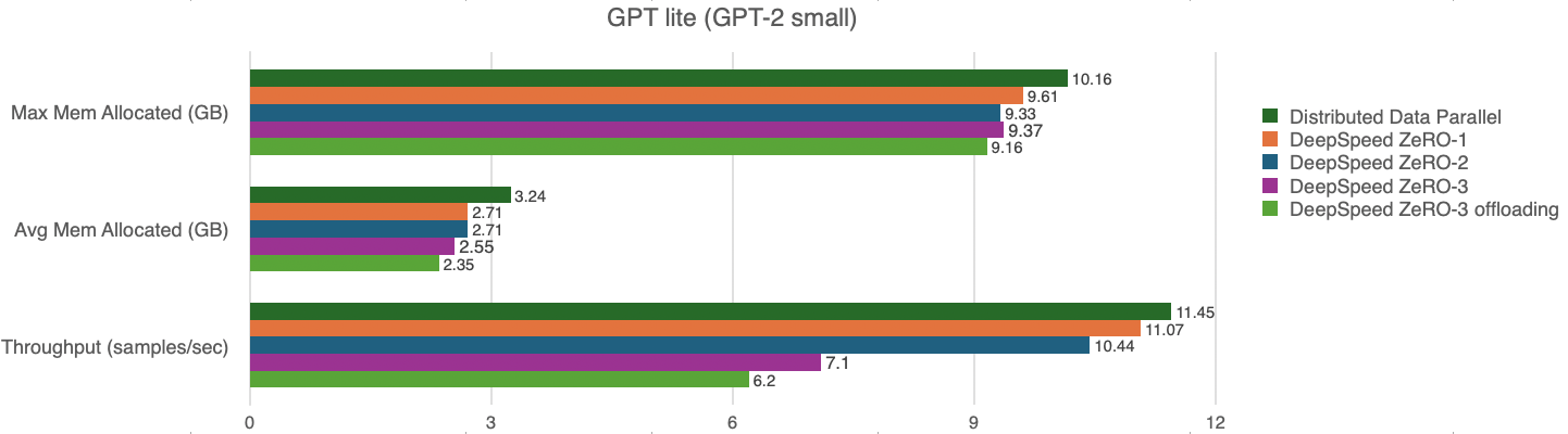
Memory overhead from communication buffers. Looking at the max vs average memory, note that the max memory in theory should be much higher at high ZeRO stages compared to low ZeRO stages and DPP. This is due to more parameters being communicated requiring more communication buffers. However, setting the communication bucket sizes to a low value in the config file overcomes this effect. In fact, we also benchmarked several runs with the default communication bucket sizes (5e9) and it led to a higher memory usage as expected (of approximately double the amount in stages 2 and 3), that became prohibitive for some runs.
Communication vs computation trade-off from different stages in ZeRO. In ideal scenarios, as you move from DDP to ZeRO-1, ZeRO-2, ZeRO-3 and ZeRO-Infinity, the memory consumption and throughput are reduced. As expected, we swap data locality for communication of parameters, and pay a price in performance for the communication/offload of parameters.
Offloaded vs in-memory parameters. Offloading proved to be a consistent way to reduce memory usage with the drawback of a small reduction of throughput, as expected.
Lack of superlinear speedup: We observed a small improvement of memory efficiency, but still far from the claims of the original DeepSpeed team. One explanation is that we used a small network of 8 GPUs, compared to the 64 to 800 GPUs used by the authors in their benchmarks, therefore we achieved a much smaller memory reduction. A large network of GPUs also underlies their claim of superlinear speed up that we did not observe.
Finally, we did not use communication quantization as did not result in any improvement. This goes in line with the ZeRO++ paper where it claims this method is applicable for small batch sizes or low-latency / low-bandwidth networks.
Resources and code
In this post we explored only the dimension of data parallelism. If you’d like to know more about DeepSpeed, check the DeepSpeed API documentation, the training features page, the tutorials page, the HuggingFace page for DeepSpeed, and the examples at DeepSpeedExamples.
There are a lot of results and food for thought here, so I will update this post as I find new insights. Meanwhile, if you want to try this on your own, see the GPT-lite-distributed repo.