Distributed training of variable-length samples: curriculum learning, compilation, adaptive batch size and LR
Many datasets include samples of variable length—for example, audio tracks of different durations, text sentences with different numbers of tokens, and videos with different numbers of frames. To train a machine learning model on such data, it is common to trim and pad all samples to a fixed length so batch shapes are consistent across training iterations. Alternatively, you can train on the original sample sizes, which adds complexity—especially in distributed (multi-node, multi-GPU) environments.
In this post, we introduce and implement three techniques that accelerate training with variable-length inputs in multi-process runs: (1) curriculum learning to make the model learn faster and more stably, (2) adaptive batch size and learning rate to better utilize hardware by allowing large batches of short samples (and vice versa) with a corresponding learning-rate adjustment, and (3) static kernel compilation to reduce runtime overhead.
Curriculum Learning
Curriculum learning is a training method that presents samples to the model in order of increasing difficulty (e.g., increasing noise level, increasing human score, or increasing length). This can improve stability and final performance. The rationale is that presenting very difficult samples early in training can produce large gradients and abrupt parameter updates, which may destabilize learning. Presenting samples in increasing difficulty tends to yield a smoother and more stable learning process.
Curriculum learning can also improve efficiency for variable-length data. Mixing short and long sequences in the same batch forces padding up to the longest sequence, which adds substantial compute and memory overhead.
At a high level, curriculum learning is simple: (1) define a difficulty metric per sample, (2) sort samples by increasing difficulty, and (3) iterate through the sorted dataset. In distributed runs with large datasets, however, this becomes non-trivial. Samples are typically assigned to ranks in an interleaved fashion (e.g., via PyTorch’s DistributedSampler), which can lead to load imbalance if each rank sorts only its local shard—illustrated as (a) and (b) below.
An illustration of the curriculum dataset setup problem on a network of 4 ranks and a dataset of 16 samples.
There are two main approaches:
- Simple (but potentially imbalanced and non-deterministic): each rank loads its shard, sorts locally, and applies curriculum learning on its local order (diagram (c)). This can cause load/runtime imbalance and makes results dependent on the number of ranks.
- Complex (but balanced and deterministic): perform a distributed sort across all ranks (diagram (d)), then reassign the globally sorted dataset in an interleaved fashion (diagram (e)). This yields an almost perfectly balanced distribution across ranks (diagram (f)).
In the next sections we detail the latter option.
Distributed Sorting
The tricky part is the distributed sort that transforms (b) into (d). There are other distributed sorting algorithms one could use, but here we implement the Distributed Sample Sort algorithm because it scales well to many processes. The workflow is:

A Python implementation is provided below.
def sample_sort(tensor, comm_group, num_workers, n_samples=100):
    # Perform a distributed sample sort of a tensor and return this rank's sorted shard.
    device, dims = tensor.device, tensor.size()[1]

    # 1 - sort rows lexicographically (by col0, then col1, ...)
    tensor = torch.tensor(sorted(tensor.tolist()), dtype=tensor.dtype, device=tensor.device)

    # 2 - collect a few samples per rank (use the first column as key)
    idx = torch.round(torch.linspace(0, len(tensor) - 1, n_samples)).to(int)
    samples = tensor[idx][:, 0].contiguous().to(device)

    # 3 - all-gather samples
    all_samples = [torch.zeros(n_samples, dtype=samples.dtype, device=device) for _ in range(num_workers)]
    dist.all_gather(all_samples, samples, group=comm_group)
    all_samples = torch.cat(all_samples, dim=0).to(device)

    # 4 - sort all samples and choose range boundaries for each rank
    all_samples = all_samples.sort()[0]
    idx = torch.round(torch.linspace(0, len(all_samples) - 1, num_workers + 1)).to(int)
    ranges = all_samples[idx]  # rank r owns: ranges[r] <= x < ranges[r+1]
    ranges[-1] += 1  # ensure the last bucket includes the max value

    # 5 - bucket local rows by their key range
    send = []
    for rank in range(num_workers):
        mask = (tensor[:, 0] >= ranges[rank]) & (tensor[:, 0] < ranges[rank + 1])
        send.append(tensor[mask])

    # 6 - all-to-all to communicate send/recv sizes (in number of scalars)
    send_count = [torch.tensor([len(s) * dims], dtype=torch.int64, device=device) for s in send]
    recv_count = list(torch.empty([num_workers], dtype=torch.int64, device=device).chunk(num_workers))
    dist.all_to_all(recv_count, send_count, group=comm_group)

    # 7 - all-to-all-v to exchange the flattened payloads
    send = torch.cat(send, dim=0).flatten().to(device)
    recv = torch.zeros(sum(recv_count), dtype=send.dtype).to(device)
    send_count = [s.item() for s in send_count]
    recv_count = [r.item() for r in recv_count]
    dist.all_to_all_single(recv, send, recv_count, send_count, group=comm_group)
    del send

    # 8 - reshape and sort locally again
    recv = recv.view(-1, dims)
    recv = torch.tensor(sorted(recv.tolist()), dtype=recv.dtype, device=recv.device)
    return recv
If you are interested in the remaining code, check my DeepSpeed PR 5129, which includes support utilities (e.g., writing the post-sorting distributed tensor in (d) to a sequential file via file_write_ordered).
Adaptive batch size and learning rate
When training variable-length datasets, it is common to batch by token count instead of by sample count—i.e., group samples so the sum of sequence lengths in the batch stays near a target. For example, in Attention is all you need, section 5.1:
Sentence pairs were batched together by approximate sequence length. Each training batch contained a set of sentence pairs containing approximately 25000 source tokens and 25000 target tokens.
This helps equalize work across batches (and across ranks). It is also particularly relevant for curriculum learning: a batch with shape B x T x E (batch size × sequence length × embedding size) will often have high B and low T early in the curriculum (many short samples), and low B and high T later (fewer long samples).
However, varying the batch size B typically requires adjusting the learning rate (LR). Two widely used scaling rules are:
- Linear scaling: when the minibatch size is multiplied by
k, multiply the LR byk(e.g., Accurate, Large Minibatch SGD: Training ImageNet in 1 Hour, Goyal et al.). - Square-root scaling: when the minibatch size is multiplied by
k, multiply the LR bysqrt(k)to keep gradient noise roughly constant (e.g., One weird trick for parallelizing convolutional neural networks, Krizhevsky et al.).
In practice, the hyperparameters are: (1) a target token count per batch, (2) a reference learning rate, and (3) a reference batch size. During training, each batch is packed until it reaches the token budget, and LR is scaled based on the realized batch size.
Illustrative example
Assume a limit of \(30\) tokens per batch, a reference LR of \(10^{-3}\), and a reference batch size of \(2\). Early in curriculum learning (short sequences), batches will contain more samples than later (long sequences), as shown below:
Here, samples are collected until the batch reaches (at most) 30 tokens. The batch sizes (number of samples) become \(10\) and \(4\) in the left and right examples, respectively. Using linear scaling, the corresponding LRs are \(5 imes 10^{-3}\) and \(2 imes 10^{-3}\).
Pipeline parallelism
Pipeline parallelism
requires the same batch size and sequence length across all micro-batches within a batch, because activation shapes must stay fixed during gradient accumulation. Enforcing a consistent B x T x E across micro-batches can lead to smaller micro-batches and additional padding. The figure below contrasts standard Distributed Data Parallel (DDP, left) with pipeline parallelism (right) for 2 processes and 2 gradient accumulation steps (4 micro-batches total):
In the pipeline case (right), all micro-batches in the batch have the same B x T x E shape. To satisfy this constraint, fewer samples are packed per micro-batch compared to the non-pipeline case (left), and padding is used when needed.
Attention matrix
Attention is a particular challenge in variable-length training. With fixed shapes, an input of shape B x T x E often uses a 2D attention mask of shape T x T, broadcast over the batch dimension. With variable lengths, we need a per-sample mask, which is naturally represented as a B x T x T tensor. For example, for the non-pipeline micro-batch 1 above (top-left; 4 sentences), the mask can be illustrated as:
A useful way to think about the cost is that attention scales linearly with B and quadratically with the maximum T in the batch. Allowing T to vary (and adapting B accordingly) can therefore improve utilization by avoiding padding to an unnecessarily large T.
Implementation
Variable learning rate is implemented as a scheduler wrapper that scales the LR of an underlying scheduler at each step based on the realized batch size:
class VariableBatchSizeLR(LRScheduler):
    # An LR scheduler wrapper that scales LR based on the realized batch size.

    @property
    def optimizer(self):
        return self.base_lr_scheduler.optimizer

    def __init__(self, lr_scheduler, base_batch_size, batch_sizes, dataloader,
                 lr_scaling_method="linear", last_epoch=-1, verbose=False):
        self.batch_sizes = batch_sizes
        self.base_batch_size = base_batch_size
        self.lr_scaling_method = lr_scaling_method
        self.dataloader = dataloader
        self.base_lr_scheduler = lr_scheduler
        self.base_lrs = self.base_lr_scheduler.get_lr()
        self.last_epoch = last_epoch
        self.verbose = verbose
        self.step(0)

    # [...]

    def step(self, epoch=None):
        # call the base scheduler's step method to get LR for next epoch
        # Note: optimizer.step() precedes lr_scheduler.step(), so:
        # init: lr_scheduler.step(0) --> set LR for epoch 0
        # epoch 0: optimizer.step(); lr_scheduler.step(1) --> set LR for epoch 1
        # epoch 1: optimizer.step(); lr_scheduler.step(2) --> set LR for epoch 2

        # reset unscaled LRs (to the base scheduler's values) for the current epoch
        # Note: epoch==0: reset LR scheduler; epoch==None: scale LR for next epoch;
        unscaled_lrs = self.base_lrs if epoch == 0 else self.get_last_lr()
        for group, lr in zip(self.base_lr_scheduler.optimizer.param_groups, unscaled_lrs):
            group['lr'] = lr

        self.base_lr_scheduler.step(epoch)

        # scale the learning rate for the next epoch for each parameter group
        self.last_epoch = self.last_epoch + 1 if epoch is None else epoch
        batch_size = self.batch_sizes[self.last_epoch % len(self.batch_sizes)]
        for group in self.base_lr_scheduler.optimizer.param_groups:
            group['lr'] = scale_lr(self.base_batch_size, batch_size, group['lr'], self.lr_scaling_method)
Adaptive batch size is implemented as a data loader with a special collate function that packs samples into token-budgeted micro-batches:
def dataloader_for_variable_batch_size(dataset, microbatch_ids, batch_max_seqlens,
    dataloader_rank=0, dataloader_batch_size=1, dataloader_num_replicas=1,
    dataloader_collate_fn=None, dataloader_num_workers=2, dataloader_pin_memory=False,
    required_microbatches_of_same_seqlen=False, sample_padding_fn=None,
):

    # Equidistantly distribute the microbatches across replicas (interleaved).
    sampler = DistributedSampler(
        dataset=microbatch_ids,
        num_replicas=dataloader_num_replicas,
        rank=dataloader_rank,
        shuffle=False,
        drop_last=False,
    )

    # Wrap the user-defined collate function to handle variable-batch packing.
    def collate_fn_wrapper(list_microbatch_ids):
        # Each batch element is a list of sample ids that fills up to max tokens.
        # We return the collated batch over all dataset samples referenced in the microbatches.
        batch = []
        for batch_id, microbatch_ids in list_microbatch_ids:
            batch_data = [dataset[idx] for idx in microbatch_ids]
            if required_microbatches_of_same_seqlen:
                assert sample_padding_fn is not None,                     "sample_padding_fn must be provided if required_microbatches_of_same_seqlen is True"
                pad_len = batch_max_seqlens[batch_id]
                batch_data = [sample_padding_fn(sample, pad_len) for sample in batch_data]
            batch += batch_data
        return dataloader_collate_fn(batch) if dataloader_collate_fn else batch

    return DataLoader(
        dataset=microbatch_ids,
        batch_size=dataloader_batch_size,
        sampler=sampler,
        num_workers=dataloader_num_workers,
        collate_fn=collate_fn_wrapper,
        pin_memory=dataloader_pin_memory,
    )
If you are looking for a complete example, see my DeepSpeed PR 7104.
Kernels compilation
We have seen in a previous post that just-in-time compilation of ML kernels via torch.compile can lead to substantial speedups. Here we focus on two aspects: (1) compilation on distributed runs and CUDA graphs, and (2) static vs dynamic compilation.
CUDA graphs compilation on single- vs multi-process runs
Compilation via torch.compile uses a mode that controls optimization aggressiveness. One important optimization is compiling into a CUDA graph. CUDA graphs can capture and replay a sequence of kernels entirely on the GPU, reducing CPU overhead from kernel launches.
Consider a feed-forward network with 3 linear layers and 3 activations on a single GPU. The data loading, forward pass, backward pass, and optimizer step can be illustrated as:
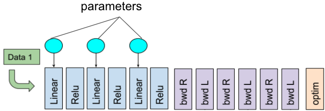
A single-GPU training iteration workflow (adapted from the original PyTorch dev discussion).
In this example, the GPU executes many separate kernels in forward/backward. If captured as a CUDA graph, those kernels can be replayed with fewer launches, which often improves throughput:
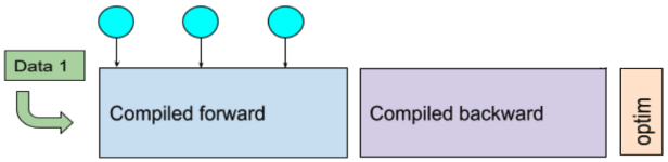
A single-GPU training iteration workflow of a compiled model (adapted from the original PyTorch dev discussion).
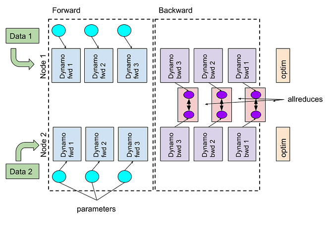
Now consider a 2-GPU Distributed Data Parallel (DDP) run. During backprop, DDP performs all_reduce operations to synchronize gradients across ranks. These collectives can overlap with gradient computation because loss.backward() accumulates into w.grad and optimizer.step() applies updates later; thus, gradients from earlier layers can be reduced while later-layer gradients are still being computed:
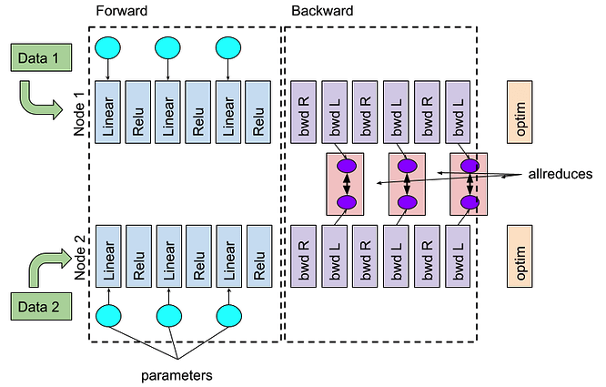
The DDP execution workflow on 2 GPUs. The optimizer needs to wait for all asynchronous all_reduces of gradients to finish (source: PyTorch dev discussion).
In a compiled setting, intermediate communication steps can introduce graph breaks. One naïve option is to compile a large graph and run the all_reduces only at the end, but that reduces overlap and increases the time the optimizer waits:
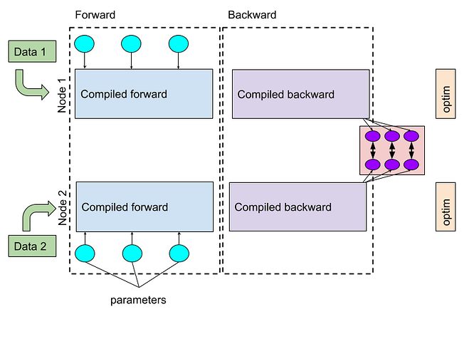
The DDP workflow on 2 GPUs with compiled models. The all_reduce runs only at the end, increasing optimizer wait time (source: PyTorch dev discussion).
PyTorch’s DDPOptimizer (explained here) addresses this by compiling around graph breaks into subgraphs and triggering asynchronous synchronization at subgraph boundaries:
The DDP workflow on 2 GPUs with compiled subgraphs and DDPOptimizer. Synchronization happens asynchronously between subgraphs (source: PyTorch dev discussion).
Note that subgraph boundaries may change with input shapes. As a personal note, I have not been able to achieve the same distributed speedups with DeepSpeed ZeRO-0 that I got with PyTorch DDP, possibly due to the lack of an equivalent optimization to DDPOptimizer in DeepSpeed.
Static compilation of variable-shaped inputs
PyTorch provides limited support for compiling variable-shaped tensors via torch.compile(dynamic=True). In practice (in my tests with torch==2.4.0), dynamic compilation was slower than static compilation and did not work reliably for both dynamic batch and dynamic sequence length.
Static compilation is ideal, but how can we make it work with variable shapes? A practical approach is to ensure that each rank executes at least one forward+backward pass for every shape it will see later, near the beginning of training—so the compiler can generate (and cache) a binary per shape. The idea is illustrated below:
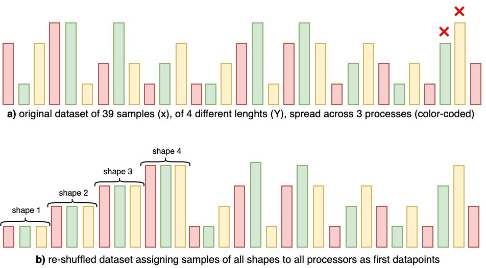
Setting up the dataset to allow static compilation for variable-length training on 3 processes. Top (a): default interleaved assignment (color-coded). The green and yellow ranks encounter a new shape later (red cross), triggering recompilation and potentially a runtime failure depending on settings. Bottom (b): reshuffling so each rank sees one sample of each shape early enables compiling one binary per shape and then running without surprises.
You can inspect compilation behavior by setting TORCH_LOGS=recompiles. For example, if the dataset contains lengths \(10\), \(20\), \(30\), and \(40\), you would see recompiles when a new length appears:
Recompiling function forward in train.py:145 triggered by the following guard failure(s):
    - tensor 'L['timestep']' size mismatch at index 0. expected 10, actual 20
and similarly for subsequent new lengths.
Keep in mind that each new shape can produce a new compiled variant that consumes memory. If the number of shapes is large, this can lead to out-of-memory (OOM) issues. Two practical mitigations are:
- Pad/bucket lengths to reduce the number of distinct shapes.
- Order inputs by size and call
torch.compiler.reset()after a set of compilations to free cached variants that will not be needed again.
Finally, pass arguments like the following to torch.compile to implement this logic:
world_size = torch.distributed.get_world_size()
mode = "max-autotune" if world_size == 1 else "max-autotune-no-cudagraphs"  # single vs multi-GPU
dynamic = False  # force static compilation
model = torch.compile(model, backend="inductor", mode=mode, dynamic=dynamic)
As a final remark, I tested this on torch==2.4.0, and newer PyTorch releases continue to improve compilation for distributed and dynamic-shape workloads. For a deeper dive, see “torch.compile the missing manual”.