Variational Inference: ELBO, Mean-Field Approximation, CAVI and Gaussian Mixture Models
We learnt in a previous post about Bayesian inference, that the goal of Bayesian inference is to compute the likelihood of observed data and the mode of the density of the likelihood, marginal distribution and conditional distributions. Recall the formulation of the posterior of the latent variable \(z\) and observations \(x\), derived from the Bayes rule without the normalization term:
\[p (z \mid x) = \frac{p(z) \, p(x \mid z)}{p(x)} \propto p(z) \, p(x \mid z) \label{eq_bayes}\]read as the posterior is proportional to the prior times the likelihood. We also saw that the Bayes rule derives from the formulation of conditional probability \(p(z\mid x)\) expressed as:
\[p (z \mid x ) = \frac{p(z,x)}{p(x)} \label{eq_conditional}\]where the denominator represents the marginal density of \(x\) (ie our observations) and is also referred to as evidence, which can be calculated by marginalizing the latent variables in \(z\) over their joint distribution:
\[p(x) = \int p(z,x) dz \label{eq_joint}\]The inference problem is to compute the conditional probability of the latent variables \(z\) given the observations \(x\) in \(X\), i.e. conditioning on the data and compute the posterior \(p(z \mid x)\). For many models, this evidence integral does not have a closed-form solution or requires an exponential time to compute.
There are several approaches to inference, comprising algorithms for exact inference (Brute force, The elimination algorithm, Message passing (sum-product algorithm, Belief propagation), Junction tree algorithm), and for approximate inference (Loopy belief propagation, Variational (Bayesian) inference, Stochastic simulation / sampling / Markov Chain Monte Carlo). Why do we need approximate methods after all? Simply because for many cases, we cannot directly compute the posterior distribution, i.e. the posterior is on an intractable form — often involving integrals — which cannot be (easily) computed. This post focuses on the simplest approach to Variational Inference based on mean-field approximation.
Detour: Markov Chain Monte Carlo
Before moving into Variational Inference, let’s understand the place of VI in this type of inference. For many years, the dominant approach was the Markov chain Monte Carlo (MCMC). A simple high-level understanding of MCMC follows from the name itself:
- Monte Carlo methods are a simple way of estimating parameters via generating random numbers. A simple example is to compute the area of a circle inside by generating random 2D coordinates whitin the bounding square around the circle, and estimate the value of \(\pi\) or the area of the circle from the proportion of generated datapoints that fall inside vs outside the circlle in the square;
- Markov Chain is a stochastic model describing a sequence of events in which the probability of moving to a next state depends only on the state of the current state and not on the previous ones; an example would be the probability of the next character in a word for all 27 possible characters, given the current character.
Therefore, MCMC methods are used to approximate the distribution (state) of parameters at a next iteration by random sampling from a probabilitistic space defined in the current state. MCMC is based on the assumption that the prior-likelihood product \(P(x \mid z) \, P(z)\) can be computed, i.e. is known, for a given \(z\). However, we can do this without having any knowledge of the function of \(z\). But we know that from a mathematical perspective (eq. \ref{eq_bayes}) the posterior density is expressed as:
\[\begin{align*} p (z \mid x) & = \frac{p(z) \, p(x \mid z)}{p(x)} & \text{(Bayes equation)} \\ & = \frac{p(z) \, p(x \mid z)}{\int p(z) p(x \mid z) \,dz} & \text{(marginalizing } z \text{)} \\ \end{align*}\]where the top term of the division can be computed, but the bottom one is unknown or intractable. Since the bottom term is a normalizer — i.e. guarantees that the posterior sums to 1, we can discard it, leading to the expression \(p (z \mid x) \propto p(z) \, p(x \mid z)\). Therefore, the rationale is that we can take several samples of the latent variables (as en example the mean \(\mu\) or variance \(\sigma^2\) in normal distribution) from the current space, and update our model with the values that explain the data better than the values at the current state, i.e. higher posterior probability. A simpler way to represent this description is to compute the acceptance ratio of the proposed over the current posterior (allowing us to discard the term \(P(x)\) which we couldn’t compute):
\[\frac{ P(z \mid x) }{ P(z_0 \mid x) } = \frac{ \hspace{0.5cm}{ } \frac{P(x \mid z) \, P(z)}{ P(x) } \hspace{0.5cm} } { \,\, \frac{P(x \mid z_0) \, P(z_0)}{ P(x) } \,\, } = \frac{ P(x \mid z) \, P(z) }{ P(x \mid z_0) \, P(z_0)}\]and perform a step change towards the state of highest ratio.
The main advantage of MCMC is that it provides an approximation of the true posterior, although there are many disavantadges on handling a exact posterior which doesn’t follow a parametric ditribution (such as hard interpretability in high dimensions). Moreover, it requires a massive computation power for problems with large latent spaces. That’s where Variational Inference enters the picture: it’s faster and works well if we know the parametric distribution of the posterior, however being sometimes over-confident when posterior are not exact to the approximated.
So as a golden rule, always use approximated methods, but if in doubt, double check with the true MCMC-based posterior.
I will try to post about this topic in the near future, but if you’re curious you can always check the paper An Introduction to MCMC for Machine Learning if you are interested on the theory behind it, or a practical explanation with code in Thomas Wiecki’s post.
Variational Inference
The idea behind Variational Inference (VI) methods is to find a parametric distribution \(q(z)\) that is an approximation of an intractable/non-parametric posterior \(p(z \mid x)\). To do that, we first define a function that gives the approximation/similarity/closeness/proximity between the two probabilities \(p\) and \(q\). So we start by defining the Kullback–Leibler (KL) divergence between two probabilities \(f(x)\) and \(g(x)\) as:
\[KL (f(x) || g(x)) = \int f(x) \log \frac{f(x)}{g(x)} dx= \mathbb{E} \left[ \log \frac{f(x)}{g(x)} \right] = \mathbb{E} \left[ \log f(x) \right] - \mathbb{E} \left[ \log g(x) \right]\]when applied to our use case:
\[KL (q(z) || p(z \mid x)) = \int q(z) \log \frac{q(z)}{p(z \mid x)} dz= \mathbb{E} \left[ \log \frac{q(z)}{p( z\mid x)} \right] \label{eq_KLdiv}\]Note that KL-divergence is a dissimilarity function and is not a metric as it’s not symmetric. And that there are other divergence metrics other than KL divergence, part of the f-divergence family.
Looking at equation \ref{eq_KLdiv}, we see an issue: it includes the true posterior \(p(z \mid x)\) which is exactly the value we do not know. So we cannot minimize this directly, but we can minimize a function that is equal to it (up to a constant), known as the Evidence Lower Bound.
Evidence Lower Bound (ELBO)
We can rewrite the KL divergence as:
\[\begin{align*} KL (q(z) || p(z \mid x)) & = \int q(z) \log \frac{q(z)}{p(z \mid x)} dz \\ & = \int q(z) \log \frac{q(z)p(x)}{p(z, x)} dz & \text{(definition of conditional prob.)}\\ & = \int q(z) \left( \log p(x) + q(z) \log \frac{q(z)}{p(z, x)} \right) dz & \text{(expanding } \log \text{)}\\ & = \log p(x) \int q(z) dz + \int q(z) \log \frac{q(z)}{p(z, x)} dz & \text{(definition of conditional prob.)}\\ & = \log p(x) - \int q(z) \log \frac{p(z, x)}{q(z)} dz & \text{(negate log; } q(z) \text{ is a dist. thus } \int q(z) dz =1 \text{)}\\ &= \log p(x) - ELBO(q,p)\\ \end{align*}\]In practice, we replaced the original \(KL\)-divergence formulation we could’t not minimize by an expression that we can minimize. Looking at the right-hand side of the expression:
- We want to minimize the KL divergence over \(q\), so the term \(\log p(x)\) can be ignored as it does not contain \(q\).
- We know all terms inside \(ELBO(q,p)\), as \(p(z,x)\) is just the prior times the likelihood \(p(z,x) = p(z) \, p(x \mid z)\), which are the inputs of the problem;
- We know that the KL can not be negative. Thus \(\log p(x) \ge ELBO\), i.e. the ELBO is always smaller than the evidence \(p(x)\), and this explains the name Evidence lower bound.
Note that ELBO can also be described as, and is usually found expressed in terms of the expectations of the two variables as:
\[ELBO(q,p) = \int q(z) \log \frac{p(z, x)}{q(z)} = \int q(z) \log p(z, x) dz - \int q(z) \log q(z) dz = \mathbb{E} [\log p(x,z)] - \mathbb{E}[\log q(z)] \label{eq_elbo}\]There are several options to solve the previous optimization problem: coordinate descent in all variables \(z_i\) (slow, and requires one to derive by hand the formulation of the gradients), Stochastic Variational Inference (faster), Mean-field approximation, etc.
Mean-field approximation
So far we foccused on a single posterior defined by a family with a single distributions \(q\), whose posterior \(p(z \mid x)\) is tractable. We now extend our analysis to complex families, where the posterior is not tractable.
One way to overcome it is to approximate the posterior probability using a simpler model. For example, assuming that a set of a set of latent variables is independent of other variables. Or we can enfurce full independence among all latent variables given \(x\). This assumption is known as the mean-field approximation.
In practice, this methods originates from mean-field theory. From wikipedia:
“Mean-field theory […] studies the behavior of high-dimensional random (stochastic) models by studying a simpler model that approximates the original by averaging over degrees of freedom. […] The effect of all the other individuals on any given individual is approximated by a single averaged effect, thus reducing a many-body problem to a one-body problem.”
More complex scenarios such as variational family with dependencies between variables (structured variational inference) or with mixtures of variational families (covered in Chris Bishop’s PRML book) will be covered in a future post. As a side note, because the latent variables are independent, the mean-field approach that follows usually does not contain the true posterior.
In this type of Variational Inference, due to variable independency, the variational distribution over the latent variables factorizes as:
\[q(z) = q(z_1, ..., z_m) = \prod_{j=1}^{m} q(z_j) \label{eq_posterior_mf}\]where each latent variable (\(z_j\)) is governed by its own density \(q(z_j)\). Note that the variational family input does not depend on the input data \(x\) which does not show up in the equation.
We can also partition the latent variables into \(K\) groups \(z_{G_1}, ..., z_{G_K}\), and represent the approximation instead as:
\[q(z) = q(z_1, ..., z_m) = q(z_{G_1}, ..., z_{G_K}) = \prod_{j=1}^{K} q_j(z_{G_j})\]This setup is often called generalized mean field instead of naive mean field. Each latent variable \(z_j\) is governed by its own variational factor, the density \(q_j(z_j)\). For the formulation to be complete, we’d have to specify the parametric form of the individual variational factors. In principle, each can take on any parametric distribution to the corresponding random variable (e.g. a combination of Gaussian and Categorical distributions).
Coordinate Ascent Variational Inference
The main objective is to optimize the ELBO in the mean field variational inference, or equivalently, to choose the variational factors that maximizes the ELBO (eq. \ref{eq_elbo}). A common approach is to use the coordinate ascent method, by optimizing the variational approximation of each latent variable \(q_{z_j}\), while holding the others fixed.
Recall the probability chain rule for more than two events \(X_1, \ldots , X_n\):
\[P(X_n, \ldots , X_1) = P(X_n | X_{n-1}, \ldots , X_1) \cdot P(X_{n-1}, \ldots , X_1)\]on its recursive notation; or the following on its general form:
\[P\left(\bigcap_{k=1}^n X_k\right) = \prod_{k=1}^n P\left(X_k \,\Bigg|\, \bigcap_{j=1}^{k-1} X_j\right)\]Remember from eq. \ref{eq_elbo} that \(ELBO(q) = \mathbb{E} [\log p(z, x)] - \mathbb{E}[\log q(z)]\). We now apply the chain rule to the joint probablility \(p(z_{1:m}, x_{1:n})\) for \(m\) variational factors and \(n\) datapoints we get:
\[%source: assets: 10708-scribe-lecture13.pdf p(z_{1:m}, x_{1:n}) = p(x_{1:n}) \prod_{j=1}^m p(z_j \mid z_{1: (j-1)}, x_{1:n})\]and we can decompose the entropy term using the mean field variational approximation as:
\[\mathbb{E}_q [ \log q(z_{1:m})] = \sum_j^m \mathbb{E}_{q_j}[\log q(z_j)]\]Inserting the two previous reductions in the ELBO equation, we can now express it for the mean field-variational approximation as:
\[%source: assets: 10708-scribe-lecture13.pdf \begin{align*} ELBO(q) & = \mathbb{E}_q [\log p(x_{1:n},z_{1:m})] - \mathbb{E}_{q_j}[\log q(z_{1:m})] \\ & = \mathbb{E}_q \left[ \log \left ( p(x_{1:n}) \prod_{j=1}^m p(z_j \mid z_{1: (j-1)}, x_{1:n}) \right) \right] - \sum_j^m \mathbb{E}_{q_j}[\log q(z_j)] \\ & = \log p(x_{1:n}) + \sum_j^m \mathbb{E}_q \left[ \log p(z_j \mid z_{1: (j-1)}, x_{1:n}) \right] - \sum_j^m \mathbb{E}_{q_j}[\log q(z_j)] \\ \end{align*}\]We now apply the coordinate ascent variational inference (CAVI), where we compute the derivative of each variational factor and alternatively update the weights towards the lowest loss acording to the factor being iterated. Before we proceed to the derivative, we introduce the notation:
\[p (z_j \mid z_{\neq j}, x) = p (z_j \mid z_1, ..., z_{j-1}, z_{j+1}, ..., z_m, x)\]where \(\neq j\) means all indices except the \(j^{th}\). Now we want to derive the coordinate ascent update for a latent variable, while keeping the others fixed, i.e. we compute \(arg\,max_{q_j} \, ELBO\):
\[\begin{align*} & arg\,max_{q_j} \, ELBO (q)\\ = & arg\,max_{q_j} \, \left( \log p(x_{1:n}) + \sum_j^m \mathbb{E}_q \left[ \log p(z_j \mid z_{1: (j-1)}, x_{1:n}) \right] - \sum_j^m \mathbb{E}_{q_j}[\log q(z_j)] \right)\\ = & arg\,max_{q_j} \, \left( \mathbb{E}_q \left[ \log p(z_j \mid z_{\neq j}, x) \right] - \mathbb{E}_{q_j}[\log q(z_j)] \right) & \text{(removing vars that don't depend on } q(z_j) \text{)} \\ = & arg\,max_{q_j} \, \left( \int q(z_j) \log p(z_j \mid z_{\neq j}, x) dz_j - \int q(z_j) \log q(z_j) dz_j \right) & \text{(def. Expected Value)} \\ \end{align*}\]To find this argmax, we take the derivative of the loss with respect to \(q(z_j)\), use Lagrange multipliers, and set the derivative to zero:
\[\frac{d\,L}{d\,q(z_j)} = \mathbb{E}_{q_{\neq j}} \left[ \log p(z_j \mid z_{\neq j}, x) \right] - \log q(z_j) -1 = 0\]Leading to the final coordinate ascent update:
\[\begin{align} q^{\star}(z_j) & \propto exp \{ \mathbb{E}_{q_{\neq j}} [ \log p(z_j \mid z_{\neq j}, x)] \} \\ & \propto exp \{ \mathbb{E}_{q_{\neq j}} [ \log p(z_j, z_{\neq j}, x)] \} & \text{(mean-field assumption: latent vars are independent)} \label{eq_CAVI}\\ \end{align}\]However, this provides the factorization or the template of the computation, but not the final form (i.e. application to a specific distribution family) of the optimal \(q_j\). The form we choose influences the complexity or easiness of the coordinate update \(q^{\star}(z_j)\).
Multivariate Gaussian Mixture Models
Credit: this section is a more verbose explanation of sections 2.1, 3.1 and 3.2 of the paper Variational Inference: A Review for Statisticians.
A Gaussian mixture model is a probabilistic model that assumes all the data points are generated from a mixture of a finite number of Gaussian distributions with unknown parameters. The problem at hand is to fit a set of Gaussian density functions to the input dataset.
Take a family of a mixture of \(K\) univariate Gaussian distributions with means \(\mu = \mu_{1:K} = \{ \mu_1, \mu_2, ..., \mu_K \}\). The means are drawn from a common prior \(p(\mu_n)\), which we assume to be Gaussian \(\mathcal{N}(\mu, \sigma^2)\). The latent space are the means \(\mu_{1:K}\) and the cluster assignments \(c_{1:n}\) for each observation \(x_i\). \(\sigma^2\) is a hyper-parameter. \(c_i\) is described as an indicator \(K-\)vector, i.e. all zeros except a one on the index of the allocated cluster. Each new observation \(x_i\) (from a total of \(n\) observations) is drawn from the corresponding Gaussian \(\mathcal{N}(c_i^T, \mu, 1)\). The model can be expressed as:
\[%source: section 2.1: https://arxiv.org/pdf/1601.00670.pdf \begin{align} \mu_k & \thicksim \mathcal{N}(0, \sigma^2), & & k=1,...,K, \\ c & \thicksim \text{Categorical} (1/K, ..., 1/K), & & i=1,...,n, \\ x_i \mid c_i, \mu & \thicksim \mathcal{N}(c_i^T \mu, 1) & & i=1,...,n. \label{eq_gmm_likelihood}\\ \end{align}\]In this case, the joint probability of the latent and observed variables for a sample of size \(n\) is:
\[p (\mu, c, x) = p(\mu) p(c,x) = p(\mu) \, \prod_{i=1}^n p(c_i) p(x_i \mid c_i, \mu) \label{eq_7_source}\]Here we applied again the probability chain rule. The latent variables are \(z=\{\mu, c\}\), holding the \(K\)-class means and the \(n\)-point class assigments. The evidence is:
\[\begin{align*} p(x) & = \int p(\mu) \prod_{i=1}^n \sum_{c_i} p(c_i) \, p(x_i \mid c_i, \mu) d\mu \\ & = \sum_c p(c) \int p(\mu) \prod_{i=1}^n p(x_i \mid c_i, \mu) d\mu \\ \end{align*}\]I.e the evidence is now a sum of all possible configurations of clusters assignment, with a computational complexity \(O(K^n)\) due to \(K\) classes that have to be assigned to \(n\) points. We can compute this previous equation, since the gaussian prior and likelihood are conjugates. However, it is still computationally intractable due to the \(K^n\) complexity.
An alternative solution is to use the mean-field approximation method we’ve discussed. We know from before (eq. \ref{eq_posterior_mf}) that the mean-field yields approximate posterior probabilities of the form:
\[q(\mu,c) = \prod_{k=1}^K q(\mu_k; m_k, s^2_k) \prod_{i=1}^n q(c_i; \varphi_i). \label{eq_variational_family}\]and re-phrasing what was mentioned before, each latent variable is governed by its own variational factor. The factor \(q(\mu_k; m_k, s^2_k)\) is a Gaussian distribution of the \(k^{th}\) mixure component, including its mean \(m_k\) and variance \(s^2_k\). The factor \(q(c_i; \varphi_i)\) is a distribution on the \(i^{th}\) observation’s mixture assignment; its assignment probabilities are a \(K-\)vector \(\varphi_i\).
So we have two types of variational parameters: (1) the Gaussian parameters \(m_k\) and \(s^2_k\) to approximate the posterior of the \(k^{th}\) component; and (2) the Categorical parameters \(\varphi_i\) to approximate the posterior cluster assignement of the \(i^{th}\) data point. We now combine the joint density of the latent and observed variables (eq. \ref{eq_7_source}) and the variational family (eq. \ref{eq_variational_family}) to form the ELBO for the mixture of Gaussians:
\[%source https://arxiv.org/pdf/1601.00670.pdf \begin{align} ELBO(m, s^2, \varphi) = & \sum_{k=1}^K \mathbb{E} \left[ \log p(\mu_k); m_k, s_k^2 \right] \\ & + \sum_{i=1}^n \left( \mathbb{E} \left[ \log p(c_i); \varphi_i \right] + \mathbb{E} \left[ \log p(x_i \mid c_i, \mu); \varphi_i, m, s^2 \right] \right) \\ & - \sum_{i=1}^n \left( \mathbb{E} \left[ \log q(c_i; \varphi_i) \right] - \sum_{k=1}^K \mathbb{E} \left[ \log q(\mu_k ; m_k, s_k^2) \right] \right) \label{eq_algo_elbo} \\ \end{align}\]The CAVI (coordinate ascent variational inference) updates each variational parameter in turn, so we need to compute both updates.
Update 1: Variational update for cluster assignment
We start with the variational update for the cluster assignment \(c_i\). Using the mean-field recipe from equation \ref{eq_CAVI}:
\[q^{\star}(c_i; \varphi_i) \propto exp \left( \log p(c_i) + \mathbb{E} [ \log p(x_i \mid c_i, \mu); m, s^2] \right).\]The first term is the log prior of \(c_i\), the same value for all values of \(c_i\): \(\log p(c_i)= \log \frac{1}{K} = \log 1 - \log K = -\log K\). The second term is the expected log probability of the \(c_i^{th}\) Gaussian density. Because \(c_i\) is an indicator vector we can write:
\[p (x_i \mid c_i, \mu) = \prod_{k=1}^K p(x_i \mid \mu_k)^{c_{ik}}\]i.e. because \(c_{ik} = \{0,1\}\), this is a multiplication of terms that are ones except when cluster \(k\) is allocated to the datapoint \(x_i\). We use this to continue the expansion of the second term:
\[\begin{align*} & \mathbb{E} [ \log p(x_i \mid c_i, \mu); m, s^2] \\ = & \sum_k c_{ik} \mathbb{E} [ \log p(x_i \mid \mu_k); m_k, s_k^2] & \text{(sum of matching assignments } ik \text{)} \\ = & \sum_k c_{ik} \mathbb{E} \left[ \log \mathcal{N}(x_i^T \mu, 1) \right] & \text{(likelihood eq. \ref{eq_gmm_likelihood})} \\ = & \sum_k c_{ik} \mathbb{E} \left[ \log \left( \frac{1}{1 \sqrt{2\pi}} \right) - \frac{1}{2} \left( \frac{x_i - \mu_k}{1} \right)^2 ; m_k, s_k^2 \right] & \text{(log of normal distribution)} \\ = & \sum_k c_{ik} \mathbb{E} \left[ -\frac{1}{2}(x_i - \mu_k)^2; m_k, s_k^2 \right] + const & \text{(removed terms that are constant with respect to } c_i \text{)} \\ = & \sum_k c_{ik} \mathbb{E} \left[ -\frac{1}{2} x_i^2 + \mu x_i -\frac{1}{2} \mu^2; m_k, s_k^2 \right] + const & \text{(decomposed square of sum)} \\ = & \sum_k c_{ik} \left( x_i \, \mathbb{E} [ \mu_k; m_k, s_k^2] - \frac{1}{2} \mathbb{E}[ \mu^2_k; m_k, s^2_k] \right) + const & \text{(removed terms that are constant with respect to } c_i \text{)} \\ \end{align*}\]The calculation requires \(\mathbb{E} [\mu_k]\) and \(\mathbb{E} [\mu_k^2]\), computable from the variational Gaussian on the \(k^{th}\) mixture component. Thus the variational update for the \(i^{th}\) cluster assignment — expressed as a function of the variational parameters for the mixture component only — is:
\[\varphi_{ik} \propto exp \left\{ x_i \, \mathbb{E} [ \mu_k; m_k, s_k^2] - \frac{1}{2} \mathbb{E}[ \mu^2_k; m_k, s^2_k \right\} \label{eq_algo_first_step}\]Update 2: Variational update for cluster mean
We now turn to the variational density \(q(\mu_k; m_k, s^2_k)\) on equation \ref{eq_variational_family}. We use again \ref{eq_CAVI} (the exponentiated log of te joint) for the mean values \(\mu_k\):
\[q(\mu_k) \propto \exp \{ \log p(\mu_k) + \sum_{i=1}^n \mathbb{E} [ \log p(x_i \mid c_i, \mu); \varphi_i, m_{k\neq}, s^2_{k\neq} ] \}\]where the term \(\varphi_{ik}\) represents as before the probabliity that the \(i^{th}\) observation comes from the \(k^{th}\) cluster, and \(c_i\) is a one-hot (or indicator) vector. The computation of the log probability follows as:
\[\log q(\mu_k) = \log p(\mu_k) + \sum_i \mathbb{E} [ \log p(x_i \mid c_i, \mu); \varphi_i, m_{\neq k}, s^2_{\neq k}] + const\\\]We will ommit this reduction, if you are looking for details, check equations 28-32 here. This calculation leads to :
\[\log q(\mu_k) = (\sum_i \varphi_{ik} x_i) \mu_k - (\frac{1}{2} \sigma^2 + \frac{1}{2} \sum_i \varphi_{ik} ) \mu_k^2 + const.\\\]In practice it means that the CAVI optimal variational density of \(\mu_k\) is a member of the Exponential Family of Distributions with sufficient statistics \(\{\mu, \mu^2\}\) and natural parameters \(\left\{\sum_{i=1}^n \varphi_{ik} x_i, -\frac{1}{2} \sigma^2 - \frac{1}{2}\sum_{i=1}^n \varphi_{ik} \right\}\). For a detailed discussion on exponential family, sufficient statistics and natural parameters check the previous post for details. We can now express the updates for the mean and standard deviation we have:
\[\begin{align*} 0 & = \frac{d\, \log q(\mu_k)}{d\mu} \\ 0 & = \sum_i \varphi_{ik}x_i - 2 \left( \frac{1}{2} \sigma^2 + \frac{1}{2} \sum_i \varphi_{ik} \right) \mu_k \\ \hat{\mu_k} & = \frac{\sum_i \varphi_{ik} x_i}{1/\sigma^2 + \sum_i \varphi_{ik}}\\ \end{align*}\]We’ll refer to the final variable \(\hat{\mu_k}\) as \(m_k\), in line with the paper and to avoid confusions. Similarly, the update of the the standard deviation is:
\[s^2_k = \hat{\sigma}^2 = \frac{1}{1/\sigma^2 + \sum_i \varphi_{ik}}\\ \label{eq_algo_second_step}\]Algorithm and Vizualization
Putting it all together, the algorithm follows as:
- While ELBO has not converged:
- for all \(i \in \{1, ..., n\}\), set \(\varphi_{ik} \propto exp \left\{ x_i \, \mathbb{E} [ \mu_k; m_k, s_k^2] - \frac{1}{2} \mathbb{E}[ \mu^2_k; m_k, s^2_k \right\}\) (equation \ref{eq_algo_first_step})
- for \(k \in \{1, ..., K\}\) do:
- set \(m_k \leftarrow \frac{\sum_i \varphi_{ik} x_i}{1/\sigma^2 + \sum_i \varphi_{ik}}\) (equation \ref{eq_algo_second_step})
- set \(s^2_k \leftarrow \hat{\sigma}^2 = \frac{1}{1/\sigma^2 + \sum_i \varphi_{ik}}\) (equation \ref{eq_algo_second_step})
- compute \(ELBO(m, s^2, \varphi)\) (equation \ref{eq_algo_elbo})
The algorithm is iterative and will converge on a certain loss threshold (ELBO), based on the fitting of each Gaussian to the data points. The concept can be easily understood by looking at the illustration of several iterations of the fitting of Gaussian models to 4 clusters of points:
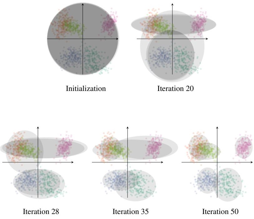
Example of the application of the CAVI algorithm to Gaussian Mixture Models. Dataset described by 2D points assigned to five color-coded clusters. (source: Variational Inference: A Review for Statisticians)
Stochastic Variational Inference
The coordinate ascent variational inference method presented does not scale well for very large datasets. The underlying reason is that CAVI requires iterating between re-analyzing every data point in the data set and re-estimating its hidden structure. This is inefficient for large data sets, because it requires a full pass through the data at each iteration.
Another famous method – Stochastic Gradient Descent (SVI) — utilizes a more efficient algorithm by using stochastic optimization (Robbins and Monro, 1951), a technique that follows noisy estimates of the gradient of the objective.
SVI is in fact stochastic gradient descent applied to variational inference. It allows the algorithm to scale to large datasets that are encountered in modern machine learning, since the ELBO can be computed on a single mini-batch at each iteration.
When used in variational inference, SVI iterates between subsampling the data and adjusting the hidden structure based only on the subsample, making it more efficient than traditional variational inference. For this reason, several ML libraries such as pyro use SVI.
I will ommit details for now, and add them when time allows. If you are interested, have a look at section 4.3 of the paper Variational Inference: A Review for Statisticians.