Publications bookmark
A summary of some interesting publications I came across. Continuously updated. Click \(\small{\blacktriangleright}\) to expand.
2026 FlashAttention-4: Algorithm and Kernel Pipelining Co-Design for Asymmetric Hardware Scaling, Princeton (Tri Dao et al.)
FlashAttention-4 (FA4) re-designs the attention kernel for NVIDIA Blackwell (B200/GB200) to confront what the authors call asymmetric hardware scaling: from Hopper to Blackwell, tensor-core (matmul) throughput jumped from ~1 to ~2.25 petaFLOPS, but the units that do everything else—the exponential unit for softmax, shared-memory bandwidth—did not speed up proportionally. The consequence is a bottleneck flip from earlier FlashAttention versions: on Blackwell the tensor cores got much faster but the exponential unit (MUFU.EX2) did not, so softmax is no longer “just the thing between the two matmuls”—it becomes the bottleneck that must be carefully pipelined. FA4’s whole job is to keep those over-provisioned tensor cores busy by overlapping the matmuls with the now-relatively-slow softmax and memory work.
The co-design has a few moving parts. New forward and backward software pipelines exploit Blackwell’s fully asynchronous MMA and larger tile sizes to overlap tensor cores, the softmax exponential, and memory operations. To beat the exponential bottleneck specifically, the forward pass emulates the exponential in software via a polynomial approximation on the FMA units, plus conditional (selective) online-softmax rescaling that only rescales when a new max actually shifts the result enough to matter. On the backward pass, where shared-memory traffic dominates, FA4 stores intermediate results in Blackwell’s new tensor memory (TMEM) to relieve shared-memory traffic, and uses the new 2-CTA MMA mode to cut shared-memory traffic and atomic reductions further. It’s also written entirely in CuTe-DSL (Python), giving 20–30× faster compile times than C++ template approaches while keeping full expressivity, which lowers the barrier to prototyping new attention variants.
Results: up to 1605 TFLOPs/s on B200 BF16 (71% utilization), 1.3× faster than cuDNN 9.13 and 2.7× faster than Triton—2–3× over FlashAttention-3, bringing attention close to raw matmul speed and effectively pushing the bottleneck back onto memory and communication. This is the kernel-level companion to the systems papers above: where they reshape what runs where, FA4 squeezes the attention primitive itself to the hardware’s asymmetric limits.
2025 LatentMoE: Toward Optimal Accuracy per FLOP and Parameter in Mixture of Experts, NVIDIA
In Nvidias LatentMoe, “tokens are projected from the model hidden dimension d into a smaller latent dimension ℓ for expert routing and computation, which reduces routed parameter loads and all-to-all traffic by a factor of d/ℓ. We use this efficiency to increase the total number of experts and the top-k active experts per token by the same factor d/ℓ”. The weighted sum of outputs (from the combined all-to-all) from all experts follows a converse projection that projects the smaller latent dimension into the original model hidden dimension, and then it’s summed with the shared experts output that do not have a dimensionality reduction. There’s only a single upward and downward projection across all experts, reducing memory bandwidth. As a side note, shared experts operate at the original model hidden space, ie without dimensionality down- and upward. They show expert computation to be restrained by HBM and then compute, in line with the max theoretical value of the roofline model.
The payoff is that the freed budget can be spent on more, finer experts at the same cost: against a standard MoE scoring 48.30% on MMLU-Pro, a LatentMoE configuration with (N’, K’) = (512, 22) reaches 52.87% on MMLU-Pro and 55.14% on code (+3.19%) at similar runtime and FLOP count. Validated by design-space exploration up to 95B parameters over a 1T-token horizon, LatentMoE consistently beats standard MoE on accuracy per FLOP and per parameter, and has been adopted by the flagship Nemotron-3 Super and Ultra models.
2025 NVIDIA Nemotron 3: Efficient and Open Intelligence, NVIDIA
Nemotron 3 (NVIDIA) is a family of open models: Nano, Super and Ultra with a context of up to 1M tokens.
The report stacks four efficiency techniques:
- LatentMoE: publication LatentMoE.
- hybrid Mamba-Transformer MoE, for inference efficiency: rather than interleaving MoE layers with expensive self-attention—which must attend over a linearly growing KV cache during generation—Nemotron 3 predominantly interleaves MoE layers with cheaper Mamba-2 layers, which require storing only a constant state during generation, keeping just a select few attention layers. .
- Multi-Token Prediction: (Super/Ultra): predicting several future tokens adds richer training signal (~2.4% average benchmark gain) and doubles as a draft for speculative decoding—a lightweight MTP module reaches ~97% acceptance on the first two predicted tokens.
- NVFP4 4-bit training: (Super/Ultra): stable, accurate pretraining on a hybrid Mamba-MoE for up to 25T tokens, with weights, activations, and gradients quantized to NVFP4 so the fprop, dgrad, and wgrad GEMMs all run in FP4 (3× peak throughput vs FP8 on GB300). The recipe leans on 2D block scaling for weights, Random Hadamard Transforms on wgrad inputs, stochastic rounding on gradients, and keeping the last 15% of the network in high precision; sensitive layers are protected too—QKV/attention projections (the few GQA layers use only 2 KV heads) stay in BF16, and Mamba output projections, which flush up to 40% of values to zero in NVFP4, are kept in MXFP8. The loss gap stays under 1% vs BF16 on Nano and shrinks to under 0.6% on the 8B-active model, with the gap narrowing as model size grows.
The design philosophy is a balance of three layer types: MoE for sparse parameter scaling, a few attention layers for high-fidelity all-to-all routing, and Mamba-2 for fixed-cost sequence modeling. Nemotron 3 Nano 30B-A3B achieves 3.3× higher throughput than Qwen3-30B-A3B, while staying competitive on reasoning and long-context (RULER @ 1M) benchmarks.
2025 Comet: Fine-grained Computation-communication Overlapping for Mixture-of-Experts, ByteDance
The standard technique for distributed MoE efficienty is to pipeline that communication with computation. Comet argues existing schemes do it too coarsely: the reason is a granularity mismatch of an MoE op into a few big chunks to expose overlap either leaves communication exposed or shrinks the GEMM tiles enough to hurt kernel efficiency (the same tension FLUX identifies for tensor parallelism).
Comet works in two parts. (1) Dependency resolving: it maps out which pieces of computation depend on which pieces of communication, then schedules them into a fine-grained pipeline so each can start the moment its data is ready. (2) Adaptive workload assignment: it splits GPU resources between comm and compute, and because the best split shifts with sequence length and parallelization strategy, it tunes that split per-configuration instead of fixing it.
Authors note that the division point of how many computation vs communication SMs to be allocated depends on the model layer, input shape and level of paralllism:
“Comet’s library comprises multiple pre-compiled kernels, each with a distinct division point (of computation vs communication SM split). Prior to deployment, the optimal configuration for each setup is profiled and stored as metadata. During runtime, Comet utilizes this metadata to select the optimal kernel for execution.” As an example, if you take the MoE workflow dispatch→MatMul→MatMul→combine, it fuses dispatch→MatMul into one kernel and MatMul→combine into other, and executes communication and computation at a tile level.
The mechanism on Hopper is thread-block specialization. Comm and compute run in separate thread blocks. One fused kernel launches a fixed set of thread blocks. Each block is specialized — it’s either a comm block or a compute block, not both. Because thread blocks occupy SMs, this effectively dedicates some SM capacity to comm and the rest to compute. When you fuse comm and compute into one kernel with specialized thread blocks, the compute blocks calls device-side functions running inside the compute thread blocks of the fused megakernel. The GEMM implementation (CUTLASS) is reused unchanged.
How does it “map out” pieces of computation to communication? The idea: between a communication op and the computation op that consumes (or produces) its data, there is a shared tensor — the buffer that comm writes into and compute reads from (dispatch), or that compute writes and comm reads (combine). Comet analyzes that buffer to figure out the fine-grained dependencies. Two steps:
- Decompose the shared tensor along a specific dimension.
- Reschedule computation to match data arrival order. Now the key move, “Mapping out the dependencies” means: for each tile of the GEMM, determine which slice(s) of the shared tensor it needs, then order the GEMM’s tile traversal to consume slices in the order communication fills them.
2025 Helix Parallelism: Rethinking Sharding Strategies for Interactive Multi-Million-Token LLM Decoding, NVIDIA
Helix Parallelism targets real-time decoding when the KV history reaches multi-million tokens under a tight token-to-token latency (TTL) budget. Two bottlenecks dominate this regime: reading the FFN weights every step, and streaming the enormous KV cache from DRAM. The problem is that the standard fix for one hurts the other. Tensor Parallelism (TP) handles FFN weight reads well, but it scales poorly for attention: once the TP width exceeds the number of KV heads, the KV cache has to be duplicated across GPUs, which wastes memory bandwidth, caps parallelism, and limits batch size. Meanwhile KV DRAM reads grow linearly with batch size. No single uniform sharding strategy relieves both pressures at once—you’re forced to trade KV duplication against FFN load.
Helix Parallelism overcomes this by introducing a hybrid execution strategy that applies KV parallelism during attention to shard KV caches across GPUs, then reuses the same GPUs for TP in dense LLMs or TP×Expert Parallel (EP) in MoEs during FFN computation.
Helix changes the parallelism layout between the attention phase and the FFN phase, within a single decode step, reusing the same GPUs.
- Phase 1 — Attention, laid out as KV Parallelism (KVP). The KV cache is sharded along the sequence/token dimension. No GPU stores a duplicate of the KV cache. The algorithm is:
- The single query for the new token is broadcast to all GPUs.
- Each GPU computes attention between that query and only its local slice of the KV cache — producing a partial attention result (partial scores + a running softmax normalizer, FlashAttention-style).
- A lightweight communication step combines the partial results into the exact full attention output. This is a small reduction (the query/output is tiny; only the KV cache is huge, and that never moves). It’s exact, not approximate.
- Phase 2 — FFN/MoE, re-laid-out as Tensor Parallel. Now the same GPUs switch view. The attention output is re-sharded so the FFN runs as:
- TP for a dense model (each GPU holds a slice of the FFN weight matrices), or
- TP × Expert Parallel for an MoE (experts distributed across GPUs).
To minimize the exposed communication cost, we introduce Helix HOP-B. Helix HOP-B effectively minimizes communication overhead through batchwise overlap.
Compared to conventional parallelism approaches, Helix reduces TTL by up to 1.5x at fixed batch sizes and supports up to 32× larger batches under the same latency budget for DeepSeek-R1.
2025 TPLA: Tensor Parallel Latent Attention for Efficient Disaggregated Prefill & Decode Inference, Peking University & Tencent
TPLA fixes an incompatibility between Multi-Head Latent Attention (MLA) and tensor parallelism:
- MLA, introduced in DeepSeek-V2, compresses the key–value state into a single low-rank latent vector
cKVand caches only that, slashing KV-cache memory. - But Megatron-LM tensor parallelism (TP)—where attention heads are split across devices—every device still needs the entire
cKVto compute its heads, so the cache is replicated on each GPU. That replication erodes MLA’s whole advantage: per-device memory ends up no better than (or worse than) plain Grouped Query Attention. An existing alternative, Grouped Latent Attention (GLA), shards the latent but then each head only sees part of it, weakening representational capacity.
TPLA’s scheme partitions both the latent representation and each head’s input dimension across devices, runs attention independently on each shard, and combines the shard outputs with an all-reduce. The key difference from GLA: every head in TPLA still attends to the full latent space (the partial results are summed back together), so it keeps MLA’s full representational power while cutting the per-device KV cache.
The split is asymmetric — TPLA uses MLA for prefill and TPLA for decode — because the two phases have different bottlenecks.
-
Prefill: keep standard (reparameterized) MLA. Prefill processes the whole prompt at once, so it’s compute-bound, not memory-bound, no KV cache.
-
Decode: switch to TPLA — partition the latent across devices. Decode generates one token at a time, so it’s memory-bound: every step you must reload the entire KV cache from HBM, and that’s where MLA’s full-cKV-on-every-device replication hurts. Here TPLA changes the layout: The latent vector cKV (and each head’s input dimension) is sliced across the TP devices. Device 0 holds the first chunk of the latent, device 1 the next, etc; then each device runs attention independently on its local shard; then they sum-reduce individual contributions. Because each head’s contribution is split and then summed, every head still effectively attends to the full latent space (just computed in pieces)
On DeepSeek-V3 and Kimi-K2 at 32K context it delivers 1.79× and 1.93× speedups while holding quality on commonsense and LongBench benchmarks, and it runs on FlashAttention-3 for real end-to-end gains. The “disaggregated” framing fits the prefill/decode split: compressed latent for memory-bound decode, full-latent attention preserved for quality.
2025 PipeFill: Using GPUs During Bubbles in Pipeline-parallel LLM Training
PipeFill improves GPU utilization in pipeline-parallel LLM training by filling idle “bubble” time—often 15–30% and sometimes over 60% of a job’s allocation—with unrelated pending jobs rather than eliminating the bubbles themselves. It fits fill-job work to measured bubble durations and available memory, adds explicit pipeline-bubble instructions, and orchestrates execution inside the gaps, yielding up to 63% higher utilization with under 2% slowdown of the main job (about 2.6K extra GPUs’ worth of work on an 8K-GPU run). This makes it complementary to schedule-optimization approaches like DualPipe, 1F1B, interleaving, and ZeroBubble, which instead shrink or hide bubbles by densifying the training job’s own schedule through forward/backward and compute/communication overlap—PipeFill is a context-switching layer, not a pipeline schedule.
Good fill jobs are workloads that tolerate interruption, with batch (offline) inference being ideal: generating embeddings for a corpus or running a smaller model over a prompt backlog. Such work is chunkable to match short bubble windows, latency-insensitive so pausing is fine, and small enough in memory to fit the spare capacity PipeFill frees up. The paper also uses other DL training jobs as fill work since training is long-running and interruption-tolerant, though inference is easier to slice into bubble-sized pieces.
2025 Speculative Decoding with Blockwise Sparse Attention, MatX
This MatX article tackles a conflict that arises when you combine two popular decoding accelerators. Speculative decoding (SD) uses a small draft model to propose several tokens that the big target model then verifies in parallel, raising operational intensity (work done per byte loaded from HBM) and giving ~2× latency/throughput gains. Blockwise sparse attention—as in DeepSeek’s Native Sparse Attention (NSA) and Moonshot’s Mixture of Block Attention (MoBA)—divides the context into blocks and lets each token dynamically attend to only a subset of them, cutting the KV data moved from HBM and again raising operational intensity (important because long contexts otherwise leave modern accelerators underutilized).
“Speculative decoding (SD) and blockwise sparse attention both accelerate LLM decoding, but when combined naively, the KV cache may lose sparsity during the verification step of SD. We show that forcing all draft tokens to attend to the same subset of the context restores sparsity while preserving model quality.”
The authors show NSA models trained this way match the language-modeling quality of baseline NSA, while achieving up to 3.5× higher operational intensity during the verification step of speculative decoding. Conceptually it’s a co-design point: rather than treating SD and sparse attention as independent layers, it reshapes the sparsity pattern so the two compose efficiently.
2025 SLA: Beyond Sparsity in Diffusion Transformers via Fine-Tunable Sparse-Linear Attention
SLA targets the attention bottleneck in Diffusion Transformers (DiTs), where long generation chains make per-step latency especially costly. Instead of committing to a single approximation (pure sparsity or pure linear attention), the paper proposes a hybrid view of attention weights: some interactions are critical and must remain “exact-ish,” while many are marginal or negligible and can be approximated or dropped.
The method combines sparse attention (for the important interactions) with a linear component (to cheaply capture the broad, low-impact mass), and introduces a fine-tunable mechanism that can adapt which interactions belong to which bucket. This makes SLA behave like a “knob” between dense and approximate attention: you can dial sparsity/linearity while preserving fidelity, which helps differentiate it from static sparse masks or fixed-kernel linear attention.
In their evaluation, SLA reports large compute reductions and practical wall-clock speedups: up to 95% attention computation reduction and up to 20× attention speedup in some settings, and 13.7× attention speedup plus 2.2× end-to-end video generation speedup on Wan2.1-1.3B.
2025 DeepSeek‑V3.2‑Exp (model card & notes), DeepSeek‑AI
DeepSeek‑V3.2‑Exp is an incremental update in the DeepSeek V3 family aimed primarily at serving efficiency, especially for long-context workloads. Compared to the original DeepSeek‑V3 technical report (Dec 2024), the emphasis shifts from “how we trained it” to “how we run it cheaper”: the release focuses on lowering attention/memory costs and improving throughput without changing the core MoE transformer recipe.
The headline change is DeepSeek Sparse Attention (DSA): instead of dense attention over all tokens, the model uses a sparse scheme that combines a lightweight “indexer” with fine-grained token selection so attention is concentrated on the most relevant tokens/blocks. In effect, this trades a bit of extra bookkeeping for fewer key/value interactions at long sequence lengths, targeting better prefill efficiency and lower KV-cache pressure.
The Hugging Face release notes also call out practical serving details (recommended runtime settings, known issues/fixes, and evaluation notes). If you already have DeepSeek‑V3 deployed, treat V3.2‑Exp as a serving-oriented refresh: expect the biggest wins when context lengths are large, while short-context quality/behavior should remain close to V3.
2025 DeepCompile: A Compiler-Driven Approach to Optimizing Distributed Deep Learning Training, Microsoft DeepSpeed
DeepCompile extends the capabilities of deep learning compilers to support distributed training. “Distributed training has become essential for scaling today’s massive deep learning models. While deep learning compilers like PyTorch compiler dramatically improved single-GPU training performance through optimizations like kernel fusion and operator scheduling, they fall short when it comes to distributed workloads.”
Existing distributed training frameworks require distributed optimizations to be implemented at the PyTorch level, which limits the ability to apply compiler-style techniques like dependency analysis or operator scheduling. “The fully sharded approach, as implemented in systems like ZeRO-3 and FSDP, employs runtime optimizations such as prefetching and unsharding:
- Prefetching aims to reduce communication overhead by initiating all-gather operations earlier than the layer where the parameters are actually needed, thereby overlapping communication with computation;
- unsharding keeps parameters in their full form to reduce communication when memory permits;
DeepCompile addresses this gap by enabling compiler-level optimizations for distributed training. It takes a standard single-GPU model implementation and transforms it into an optimized multi-GPU training graph without requiring changes to the model code”. DeepCompile applies a fully sharded approach like ZeRO-3 and FSDP on top of DeepCompile, along with three optimizations: proactive prefetching, selective unsharding, and adaptive offloading.
- Proactive prefetching. To maximize overlap between communication and computation, this optimization pass initiates all-gather as early as possible, considering how available memory changes as the forward and backward passes progresses.
- Selective unsharding. This pass keeps as many parameters unsharded as possible to reduce communication overhead caused by all-gather communication, and decides which parameters to unshard based on operator-level memory profiling
- Adaptive offloading. DeepCompile offloads optimizer states such as momentum and variance used by Adam [14] to CPU memory when GPU memory is insufficient. To reduce data transfer overhead, it offloads only the amount of data that exceeds the memory limit and schedules transfers to overlap with computation.
It automatically implements distributed ZeRO-3, ZeRO-1, and offloading. Future directions include automated parallelization (sequence/tensor parallelisms), smarter memory management, and dynamic adaptation to runtime behavior.
2025 Triton-distributed: Programming Overlapping Kernels on Distributed AI Systems with the Triton Compiler
Triton-distributed extends Triton with distributed primitives so you can write kernels that compute and communicate inside the same program, rather than launching a GEMM kernel and then calling NCCL as a separate step. The paper’s mental model is “a distributed kernel is a set of asynchronous tasks” that can signal one another and use symmetric memory (NVSHMEM-style) to move data directly between GPUs.
The key difference vs “plain Triton + NCCL” is that communication becomes an explicit part of the kernel schedule: the compiler/runtime can overlap loads, math, and remote puts/gets at a much finer granularity than stream-level overlap of independent kernels. Compared to systems like Flux/TileLink that focus on specific LLM communication patterns, Triton-distributed tries to be a general programming model (primitives + compiler support) that you can reuse across operators and topologies.
Results / takeaways:
- The paper reports speedups ranging from ~1.1× to ~20.7× on a set of distributed workloads (with the larger gains typically coming from communication-heavy patterns where fine-grained overlap matters).
- It also reports ~1.3× to ~2.4× speedups on distributed MoE workloads by enabling fused compute–communication kernels rather than staging communication into separate NCCL phases.
- In practice, it’s a “make the compiler responsible for overlap” approach: you write a single kernel that contains both compute and the collective-ish data movement, and the system handles the async orchestration.
2025 TileLink: Generating Efficient Compute–Communication Overlapping Kernels Using Tile-Centric Primitives
TileLink is a step toward Flux-like performance without requiring you to hand-craft a very specialized fused kernel for each operation. It introduces a tile-centric abstraction: tensors are mapped into 2D tiles, and the system schedules computation and communication per tile (rather than per whole tensor), enabling overlap that approximates what highly tuned systems achieve.
A useful way to distinguish TileLink from nearby work:
- Flux: decomposes specific tensor-parallel LLM ops into finely sliced pieces, then fuses them into larger kernels to overlap up to “almost all” communication; highly effective, but quite tailored.
- Triton-distributed: offers low-level in-kernel primitives (symmetric memory, signals, tasks) and a general programming model.
- TileLink: sits in between—higher-level than Triton-distributed, more general and easier to program than Flux, but still explicitly models overlap at the tile schedule level.
Results / takeaways:
- The paper reports ~1.17× to ~20.76× speedups compared to a baseline that uses standard PyTorch + NCCL-style communication patterns, depending on the operator and communication intensity.
- Against Flux specifically, TileLink reports ~1.09× to ~1.14× speedups on the workloads evaluated, positioning itself as competitive with (and sometimes slightly better than) a strong hand-optimized baseline—while aiming for broader applicability and simpler programming.
2025 MegaScale-MoE: Large-Scale Communication-Efficient Training of Mixture-of-Experts Models in Production
MegaScale-MoE is a production-oriented system for communication-efficient MoE training, where the “hard part” is not just computing experts but routing tokens and moving activations/gradients at scale. The paper’s central point is that MoE training becomes dominated by many-to-many communication (e.g., all-to-all between token routers and experts), and that you need a holistic strategy (parallelism + communication scheduling + careful micro-batching) to keep GPUs busy.
How it differs from “kernel-level fusion” work (Flux / TileLink / Triton-distributed):
- MegaScale-MoE is primarily a system/runtime + parallelization strategy for end-to-end training at very large scale, not a new kernel programming model.
- It focuses on how to structure MoE training (expert placement, token routing, communication patterns, pipeline/micro-batch choices) so the cluster behaves well, even if the underlying collectives are still “standard”.
Results / takeaways (as reported):
- The paper reports up to ~2.0× end-to-end training speedup on 32K H800 GPUs, trained on ~5 trillion tokens, for a ~7.5B-parameter model.
- The headline is that communication efficiency is not a rounding error at this scale; the system-level choices can plausibly double effective throughput in real production settings.
2025 MegaScale-Infer: Serving Mixture-of-Experts at Scale with Disaggregated Expert Parallelism
MegaScale-Infer’s answer to the memory-bound performance issue during decode is Disaggregated Expert Parallelism (DEP): disaggregate the attention and expert modules, assigning them to separate GPUs, so each can scale independently with its own parallelism. Attention modules are replicated using data parallelism, while FFN modules are scaled with expert parallelism; by consolidating requests from multiple attention replicas, the GPU utilization of each expert increases significantly as the batch size per attention replica grows. In other words, many attention replicas funnel their tokens into the expert pool, restoring large per-expert batches and turning the FFNs back into efficient compute-bound work; it also allows heterogeneous deployment—cheaper/different GPUs for attention vs. experts—to cut cost. Two systems pieces make disaggregation pay off rather than stall on communication: ping-pong pipeline parallelism, which partitions a request batch into micro-batches and shuttles them between attention and FFNs so the two GPU pools stay busy and communication hides behind compute, and a high-performance M2N communication library that eliminates unnecessary GPU-to-CPU data copies, group initialization overhead, and GPU synchronization for the token dispatch/combine traffic. It targets models up to ~1.4T parameters. This is the MoE-serving analogue of the prefill/decode and attention/FFN disaggregation seen in Helix and TPLA—here the split is attention-vs-experts, exploiting sparsity to rebatch experts efficiently.
Results / takeaways (as reported):
- For a 220B MoE model on 1024 A100 GPUs, the paper reports ~2.6× to ~4.3× speedup over baseline systems.
- For a 3T MoE model on 2048 H800 GPUs, it reports ~2.9× to ~5.4× speedup.
- For online serving scenarios, it reports ~1.6× (220B / 1024 A100) and ~2.5× (3T / 2048 H800) improvements, emphasizing that the scheduling/communication choices help under realistic request patterns, not just offline throughput.
2025 Accelerating MoE Model Inference with Expert Sharding
Balmau et al. study MoE inference from a perspective that’s easy to underestimate: even if your attention path is well optimized, expert execution and routing can dominate in sparse MoE models, and naive expert placement can create large communication volume and poor load balance.
Their approach, “expert sharding,” explores splitting experts across GPUs in a way that:
- Improves memory capacity and where expert weights live,
- Trades off communication vs. replication of weights,
- Exposes when Megatron-style GEMM parallelism helps (and when it just moves the bottleneck into communication).
This work is a useful complement to MegaScale-* systems: it is more about exposing and characterizing the performance envelope of sharded experts (and showing what makes it hard), whereas MegaScale focuses on a full production stack.
Results / takeaways: the paper’s main value is the systems analysis and the evaluation of sharding strategies that highlight which communication patterns remain dominant and where more aggressive fusion/overlap could help.
2025 TransMLA: Multi-Head Latent Attention Is All You Need, Peking University & Xiaomi
TransMLA is a post-training conversion method that turns existing Conversational Question Answering (GQA) -based models (LLaMA, Qwen, Mixtral) into MLA-based ones, without retraining from scratch. The motivation is an adoption gap. The paper’s theoretical core is a proof that GQA can always be rewritten exactly as MLA at the same KV-cache budget, but not vice versa—i.e., MLA is strictly more expressive than GQA for a given cache size. That asymmetry means any GQA checkpoint can be losslessly re-expressed in MLA form and then upgraded to use the spare expressiveness MLA affords.
TransMLA exploits this in two steps. First, it equivalently converts the model’s GQA attention into MLA structure—reformulating the repeated KV heads of GQA as low-rank latent projections—producing a model directly compatible with DeepSeek’s codebase and its optimized serving stacks (vLLM, SGLang), plus features like FP8 quantization and Multi-Token Prediction. Second, because the MLA form has representational headroom GQA wasn’t using, it fine-tunes to boost quality without growing the KV cache—and this needs only ~6B tokens to match the original model across benchmarks. The payoff: compressing 93% of LLaMA-2-7B’s KV cache yields a 10.6× inference speedup at 8K context while preserving output quality. It’s the migration path that complements TPLA and Helix: rather than designing new MLA models or new sharding, TransMLA retrofits the large existing fleet of GQA models into the more efficient MLA family.
Two observations:
- For a fixed KV-cache budget, MLA is strictly more expressive than GQA.
- Inference acceleration occurs only when MLA uses a smaller KV cache.
2025 Look Ma, No Bubbles! Designing a Low-Latency Megakernel for Llama-1B
This work targets an extreme low-latency regime: single-sequence decoding for a ~1B-parameter LLM, where performance is dominated by how efficiently the GPU can stream weights from global memory. The authors argue that modern inference engines still suffer from “pipeline bubbles” because a forward pass is split into dozens to ~100 small kernels, each incurring launch/teardown costs and synchronization stalls that prevent continuous memory streaming.
Their solution is to fuse the entire forward pass into a single megakernel that effectively acts like an on-GPU interpreter: each SM executes a schedule of “instructions” (fused RMSNorm+QKV+RoPE, attention, projections, MLP pieces, etc.). They then focus on three practical problems that show up when you fuse “about a hundred” operations:
- How to program such a megakernel (an instruction abstraction + interpreter),
- How to avoid resource contention (e.g., paged shared memory to pipeline weight loads),
- How to synchronize without kernel boundaries (a lightweight counter-based scheme).
Results / takeaways (as reported):
- On an H100, they report using ~78% of available memory bandwidth and outperforming popular engines by >1.5×; they also report that vLLM and SGLang can be limited to around ~50% bandwidth in this setting.
- In their end-to-end comparison (32-token prompt, 128 generated tokens, no speculation), they report the megakernel is ~2.5× faster than vLLM and >1.5× faster than SGLang on H100.
- On B200, they report >3.5× speedup over vLLM and still >1.5× over SGLang.
- They highlight achieving a <1 ms forward pass for a 16-bit 1B+ model on H100, and <680 µs per forward pass on B200.
This sits in a different part of the design space than Flux/TileLink/Triton-distributed: it’s about eliminating kernel boundaries entirely for single-GPU low-latency inference, rather than fusing compute with distributed communication.
2025 Mirage: A {Multi-Level} Superoptimizer for Tensor Programs (OSDI 2025)
Mirage is an automatic approach to generating deeply fused tensor programs, framing kernel fusion as a superoptimization problem over “µGraphs” (small fused subgraphs that can resemble hand-designed kernels like FlashAttention). The key point is automation: rather than manually designing a megakernel or a fused attention kernel, Mirage searches a large space of fused implementations and applies multi-level transformations to find fast code.
How it differs from other “big fusion” lines:
- Compared to manual megakernels (e.g., “No Bubbles”), Mirage aims to discover aggressive fusions automatically and generate optimized implementations.
- Compared to FlashAttention-style work, Mirage is broader: it targets arbitrary tensor programs (not just attention), and can potentially find FlashAttention-like structures when they are profitable.
- Compared to compiler frameworks like TVM/XLA, Mirage emphasizes superoptimization over small fused graphs to get performance that can beat hand tuning.
Results / takeaways (as reported in the paper):
- Mirage reports speedups of ~1.03× to ~4.6× on the forward pass across evaluated workloads and baselines.
- For end-to-end training, it reports ~1.04× to ~1.14× improvements over strong, tuned baselines—smaller than the biggest kernel-level wins, but meaningful given how optimized many training stacks already are.
2025 SageAttention3: Microscaling FP8 Attention for Inference
SageAttention3 pushes the SageAttention line toward even more aggressive inference acceleration by combining microscaling FP8 with attention-specific numerical tricks, aiming to keep attention accurate while driving GPU throughput. Conceptually, it sits between “attention kernels that assume FP16/BF16” and “end-to-end quantized models”: it focuses on the attention operator itself and is designed to be dropped into existing inference stacks.
On RTX 5090, the paper reports that SageAttention3 can reach up to 7.4× the OPS of FlashAttention3 (fp16) and up to 3.3× the OPS of FlashAttention3 (fp8), while maintaining high accuracy.
2024 LoongServe: Efficiently Serving Long-Context Large Language Models with Elastic Sequence Parallelism, Peking University
LoongServe does ring attention in the prefill phase and while rotating KV tensors across GPUs, each GPU keeps a subset of KV locally so that it is automatically available during decode. When it comes to the decode step, KV cache is sharded, so they follow the regular NOT so efficient decode parallelism algorithm, which is usually the execution bottleneck on context parallelism. they overlap comp/comm with cuda streams during prefill (ring attn), but not decode: what they claim is that while one node is sending its requests, it MAY be doing matmuls for requests it receives from other GPUs -> it’s not guaranteed, it’s opportunistic.
2024 Mamba: Linear-Time Sequence Modeling with Selective State Spaces, CMU & Princeton
Mamba is the state-space model (SSM) that made a non-attention sequence model competitive with Transformers on language. SSMs keep a fixed-size recurrent state and scale linearly in sequence length, but earlier SSMs (S4) underperformed because their dynamics were fixed regardless of input. The fix is the selection mechanism: making the SSM parameters functions of the input lets the model selectively propagate or forget information depending on the current token—giving content-based reasoning. Input-dependence breaks the convolution trick, so Mamba adds a hardware-aware parallel scan (kept in SRAM, FlashAttention-style) to stay fast. Payoff: 5× higher inference throughput than Transformers, linear scaling, and Mamba-3B matching Transformers twice its size. Its constant-size state is what eliminates the growing KV cache—the property hybrids (Jamba, Nemotron-3) exploit.
Formula. An SSM maps input $x_t$ → output $y_t$ through a hidden state $h_t \in \mathbb{R}^N$. Continuous params $(\Delta, A, B, C)$ are first discretized:
\[\bar A = \exp(\Delta A), \qquad \bar B = (\Delta A)^{-1}(\exp(\Delta A) - I)\cdot \Delta B\]Then it runs as a linear recurrence (inference) or a global convolution (training):
\[h_t = \bar A\,h_{t-1} + \bar B\,x_t, \qquad y_t = C\,h_t\]In S4 these params are fixed across time (LTI). Mamba’s change: $B$, $C$, and $\Delta$ become functions of $x_t$ (the S6 selective SSM), so $(\bar A, \bar B)$ vary per token — that’s the selectivity, and what forces the scan-based instead of convolution-based compute.
2024 Jamba: A Hybrid Transformer-Mamba Language Model, AI21 Labs
Jamba (Lieber, Lenz et al., AI21) is the first production-scale hybrid interleaving Transformer attention, Mamba SSM, and MoE layers. The core trade-off it balances: the KV cache becomes a limiting factor when scaling Transformers to long contexts, and trading attention layers for Mamba layers shrinks it—since Mamba carries only a constant-size state, not a growing cache. Attention is kept sparingly (for high-fidelity recall), Mamba does the cheap long-range work, and MoE adds capacity without adding active compute.
Released config (tunable knobs): 4 blocks of 8 layers, 1:7 attention-to-Mamba ratio, MoE every other layer, 16 experts with top-2 per token → 52B total but only 12B active, fits on one 80GB GPU. The 1:7 ratio is empirical (most of attention’s quality, most of Mamba’s memory benefit). Headline win is the cache: at 256K context Jamba needs ~4GB attention cache vs 32GB for Mixtral and 128GB for Llama-2-70B, with SOTA long-context results. Jamba 1.5 later scaled the same design to 94B active / 398B total. It’s the template Nemotron-3 follows—just adding LatentMoE and NVFP4.
2024 Better & Faster Large Language Models via Multi-token Prediction, Meta (FAIR), ICML 2024
This is the paper that establishes Multi-Token Prediction (MTP) as a general training objective (Gloeckle et al., Meta). The premise is a critique of the standard recipe: LLMs like GPT and Llama are trained with a next-token-prediction loss, and the authors argue that training to predict multiple future tokens at once yields higher sample efficiency.
The model is trained with multiple “heads.” The model predicts the following n tokens using n independent output heads sitting on top of a shared model trunk, treating multi-token prediction as an auxiliary task layered on the usual objective. While the main head predicts the next token $x_{n+1}$, auxiliary heads predict $x_{n+2}, x_{n+3}$, and so on.
- Inference Trick: During generation, the model uses these auxiliary heads to produce a “draft” of the next few tokens simultaneously with the main token.
- Parallel Verification: in the next step, the model takes those guesses and runs them through its main, high-fidelity blocks in one single forward pass.
In a standard speculative decoding setup, the roles are split strictly between iterative guessing and parallel verification:
- The Draft Model (Iterative). The small model acts just like a standard LLM. It generates tokens one by one, sequentially. Process: It predicts token 1, feeds it back into itself, predicts token 2, feeds it back, and so on, until it has a “look-ahead” sequence (usually 3–5 tokens). Why: It is small enough that these multiple sequential passes are still much faster than a single pass of the large model.
- The Larger/Target Model (All at once). The large model performs a single parallel forward pass to check the draft model’s work. Process: It takes the entire sequence of drafted tokens and processes them simultaneously using a causal mask. The “Magic”: Because of how Transformers work, the large model can calculate the probability of “Token 4” being correct at the exact same time it calculates the probability for “Token 1.” Outcome: In the time it would normally take the large model to generate one token, it verifies all the drafted tokens.
MTP is used on DeepSeek-V3 and Nemotron 3: DeepSeek-V3 refined MTP into sequential, cascaded modules that preserve the full causal chain (rather than independent parallel heads), and Nemotron 3 adopts a lightweight MTP module reaching ~97% acceptance on its first two predicted tokens.
2024 DeepSeek-V2: A Strong, Economical, and Efficient Mixture-of-Experts Language Model, DeepSeek-AI
DeepSeek-V2 introduces Multi-head Latent Attention (MLA) and DeepSeekMoE—the two architectural pillars later carried into V3 and R1. It’s a 236B-total-parameter MoE model with only 21B activated per token and a 128K context. These innovations target the two big performance bottlenecks: the KV cache of vanilla Multi-Head Attention on decoding, and dense FFNs on training.
DeepSeekMoE provides the FFN: fine-grained experts plus shared experts, so strong capacity comes from sparse activation at low compute. Two main ideas:
- Shared experts: a small number ($K_s$) that every token always uses, no routing. Used for common knowledge. These aren’t clones of each other; they’re a fixed always-on set that absorbs common/general knowledge.
- Fine-grained expert segmentation. A regular MoE has $N$ experts, each a full-size FFN, and activates top-$K$. DeepSeekMoE slices each expert into $m$ smaller ones → $mN$ total experts, and activates $mK$ of them. Same total parameters, same FLOPs — but far more combinations of experts per token. Finely segmenting the experts into $mN$ ones and activating $mK$ from them allows for a more flexible combination of activated experts.
MLA uses low-rank joint compression of keys and values: rather than caching full per-head K/V (or sharing heads as in GQA/MQA), it down-projects them into a single small latent vector cKV that is the only thing cached, then up-projects back to distinct per-head K/V at compute time—keeping full-MHA expressiveness while shrinking the cache. Because RoPE can’t be absorbed through that up-projection, V2 adds the decoupled-RoPE trick: a separate set of small query dims plus one shared key carry the positional rotation, kept apart from the compressed “content” path.
Symbols: $h_t$ = token’s input hidden vector, where $t$ is the token’s position index, $n_h$ = #heads, $d_h$ = per-head dim · $d_c$ = latent (cache) dim, $d_c \ll n_h d_h$ · $d_h^R$ = small RoPE dim · $W^{D\ast}$ = down-projections (compress), $W^{U\ast}$ = up-projections (reconstruct) · superscript $C$ = content part, $R$ = RoPE part · $j \le t$ = past tokens. Compress $h_t$ into the cached latent, then reconstruct distinct per-head K/V from it at compute time:
\[c_t^{KV} = W^{DKV}\, h_t \quad (\in \mathbb{R}^{d_c},\ \text{the only cached vector}); \qquad k_t^{C} = W^{UK} c_t^{KV},\quad v_t^{C} = W^{UV} c_t^{KV}\]where $W^{DKV}$, $W^{UK}$ and $W^{UV}$ are learnt parameters that give a lower-rank transformations. Queries are also low-rank (saves activation memory, not cached):
\[c_t^{Q} = W^{DQ}\, h_t, \qquad q_t^{C} = W^{UQ}\, c_t^{Q}\]- As a side note, when comparing with the regular attention, where the $W$ projections also give a lower-rank matrix: regular attention factors $W^K$ by head (and stays full-rank overall); MLA factors $W^K$ through a shared low-dim latent (and goes deliberately rank-deficient) — and that latent is the thing the KV cache stores.
- Note on notation: $W^{DKV}$: Down projection on KV. $W^{UK}$ and $W^{UV}$: Up projection on K and V.
Decoupled RoPE — position rides a separate path: per-head rotary queries and one shared rotary key:
\[q_t^{R} = \mathrm{RoPE}(W^{QR}\, c_t^{Q}), \qquad k_t^{R} = \mathrm{RoPE}(W^{KR}\, h_t)\]Final per-head query/key concatenate content + rotary parts:
\[q_{t,i} = [\,q_{t,i}^{C}\,;\,q_{t,i}^{R}\,], \qquad k_{t,i} = [\,k_{t,i}^{C}\,;\,k_t^{R}\,]\]Then attention is standard:
\[o_{t,i} = \sum_{j \le t} \mathrm{softmax}_j\!\left(\frac{q_{t,i}^\top k_{j,i}}{\sqrt{d_h + d_h^R}}\right) v_{j,i}^{C}, \qquad u_t = W^{O}\,[\,o_{t,1};\dots;o_{t,n_h}\,]\]KV cache per token
| MHA | GQA | MQA | MLA |
|---|---|---|---|
| $2\,n_h\,d_h$ | $2\,g\,d_h$ | $2\,d_h$ | $d_c + d_h^R$ |
The “absorb” trick folds $W^{UK}$ into $W^{UQ}$ and $W^{UV}$ into $W^{O}$ at decode time, so attention runs directly against cKV and the full per-head K/V are never materialized. DeepSeek-V2 settings: $d_c = 512$, $d_h^R = 64$ ($d_h = 128$) → cache $= 576$ scalars/token, comparable to GQA with ~2.25 groups but with full-MHA expressiveness.
Improvements over the earlier dense DeepSeek 67B are concrete: 42.5% lower training cost, a 93.3% smaller KV cache, and up to 5.76× higher maximum generation throughput, while improving quality.
2024 SageAttention2: Efficient Attention with Thorough Outlier Smoothing and Per-thread INT4 Quantization
SageAttention2 builds on SageAttention by moving to INT4 quantization for the expensive (QK^\top) path (at a thread-level granularity) while using FP8 for the \,(\widetilde{P}V)\, product. The key idea is that attention has quantization pathologies that don’t show up as strongly in linear layers—especially outliers—so the paper adds attention-specific techniques to make low-bit arithmetic viable.
Concretely, it proposes (1) per-thread INT4 quantization for (Q,K), (2) a smoothing method for (Q) to improve INT4 (QK^\top) accuracy, and (3) a two-level accumulation strategy to improve FP8 (\widetilde{P}V) accuracy. The paper reports that on RTX 4090, SageAttention2’s OPS surpasses FlashAttention2 and xFormers by about 3× and 4.5×, respectively, and that it can match FlashAttention3(fp8) speed on Hopper while achieving higher accuracy.
2024 SageAttention: Accurate 8-Bit Attention for Plug-and-play Inference Acceleration
SageAttention is an “attention-first” quantization paper: rather than quantizing an entire model, it targets the attention kernel and aims to make it plug-and-play for existing LLM inference. The motivation is that, even when linear layers are heavily optimized, attention can remain a major bottleneck—especially at long sequence lengths—because it mixes GEMMs, softmax, and reductions in ways that amplify numerical outliers.
The core idea is to run attention with 8-bit arithmetic while preserving accuracy via attention-aware scaling/handling of outliers (the paper emphasizes that naïvely quantizing (QK^\top) tends to break). Compared to later SageAttention2/3, this first version is less aggressive (INT8-style rather than INT4/FP8 microscaling) and functions as the baseline that demonstrates the feasibility of attention quantization with minimal integration work.
For performance, the paper reports substantial throughput gains on consumer GPUs: on RTX 4090, SageAttention achieves up to 8.4× higher OPS than FlashAttention2 (and up to 11.5× over xFormers), and peaks at 983 TOPS (head dim 128).
2024 Centauri: Enabling Efficient Scheduling for Communication–Computation Overlap in Large Model Training via Communication Partitioning
Centauri tackles communication–computation overlap at the operator scheduling level. The core idea is to decompose operators and then schedule the decomposed pieces across multiple CUDA streams so that communication can be overlapped with useful compute more consistently than “whole-operator overlap.” The “communication partitioning” framing highlights that a large collective (or data movement phase) can be broken into smaller chunks that are scheduled earlier and more frequently, improving pipeline utilization.
How to situate Centauri relative to Flux / TileLink / Triton-distributed:
- Centauri is mainly about multi-stream scheduling of decomposed operators and improving overlap among (still separate) kernels; it does not require in-kernel collectives.
- Flux/TileLink/Triton-distributed pursue in-kernel fusion of compute and communication, which can overlap at a finer granularity, but often requires more specialized codegen/primitives.
- Centauri is therefore a good fit when your bottleneck is orchestration (stream scheduling, dependencies, coarse kernel granularity), whereas Flux-like approaches target cases where overheads persist even with aggressive stream overlap.
Results / takeaways: the paper reports substantial training speedups on Llama-scale workloads by improving overlap through decomposition + scheduling. (If you end up writing your own fused kernels later, Centauri is still useful as a baseline: it shows what you can get “for free” from better scheduling alone.)
2024 FLUX: Fast Software-based Communication Overlap on GPUs Through Kernel Fusion
Flux is explicitly designed around Megatron-LM-style tensor-parallel patterns. Instead of treating tensor-parallel layers as “one big GEMM + one big NCCL collective,” Flux decomposes those operations into fine-grained pieces (e.g., tiles/chunks) and then fuses them into kernels that can overlap communication with computation aggressively—claiming overlap levels that are hard to reach with standard multi-stream overlap of separate kernels.
The most useful way to think about Flux in the related-work landscape:
- Compared to Centauri, Flux aims for overlap within the operator, not just between independent kernels.
- Compared to Triton-distributed, Flux is less about a general programming model and more about delivering peak performance for a specific family of LLM ops (Megatron tensor-parallel attention/MLP patterns).
- TileLink is motivated partly by Flux’s effectiveness: it tries to preserve Flux-like performance while raising the programming level.
Results / takeaways (as reported):
- Flux reports up to ~96% communication overlap.
- For Megatron-LM Llama-style inference, it reports up to ~1.66× speedup for prefill and ~1.3× for decoding.
- For training, Flux reports ~1.2× to ~1.5× speedups for Llama-3 8B pretraining, evaluated on 8-node and 3–5 node clusters with 8 GPUs per node (e.g., 24–64 GPUs total).
2024 Optimizing Distributed ML Communication with Fused Computation–Collective Operations
Punniyamurthy et al. focus on identifying common “compute + collective” motifs that appear repeatedly in distributed training/inference graphs and then implementing them as single fused kernels with in-kernel collectives. The contribution is partly a taxonomy (“these patterns show up everywhere”) and partly a concrete engineering result: implementing fused kernels in Triton/HIP that reduce overheads from intermediate writes, kernel boundaries, and separated communication steps.
The paper’s patterns are especially useful to keep in mind when comparing systems:
- Flux is very focused on tensor-parallel LLM patterns; this paper’s catalog is broader (e.g., embedding + all-to-all, GEMV + all-reduce, GEMM + all-to-all).
- Triton-distributed/TileLink offer programming models to build such fused kernels; this paper provides hand-built instances and measurements that show why the fusion matters.
- Unlike INC/offload approaches, these fused kernels still assume the communication happens through GPU-side primitives (no in-network execution).
Results / takeaways (as reported):
- The paper reports latency reductions of about 29% for embedding + all-to-all, 26% for GEMV + all-reduce, and 35% for GEMM + all-to-all, showing that the win can be material even for “simple” two-stage pipelines when communication is tightly coupled to the compute.
2024 DeepSeek-V3 Technical Report (includes DualPipe)
DeepSeek-V3 is a large-scale LLM system report that’s useful to read as a “what it takes in practice” reference: model architecture decisions, training stack choices, and the kinds of engineering trade-offs that are often omitted from purely algorithmic papers. The details are particularly relevant in a related-work section that discusses communication-heavy structures (like MoE) and the real limits of standard communication substrates.
Where it fits in the landscape here:
- DeepSeek-V3 demonstrates that you can hit strong scaling and quality with careful MoE architecture/routing and training practices, but it largely relies on standard collectives/communication stacks rather than pushing compute–communication fusion into the kernels or the network.
- This makes it a good “control point” when discussing what incremental improvements from fused kernels or in-network compute might buy: you can compare against a strong end-to-end system that already works at scale.
Results / takeaways: the report is a systems-and-training reference more than a single “one trick” optimization; it’s most valuable for its end-to-end design and empirical scaling observations, which help ground discussions about where communication becomes dominant and what kinds of optimizations remain on the table.
DualPipe is a bidirectional pipeline-parallelism algorithm introduced in the DeepSeek-V3 Technical Report, designed to reduce pipeline bubbles while addressing the heavy communication overhead of cross-node expert parallelism (which gives DeepSeek-V3 a roughly 1:1 compute-to-communication ratio). Its core idea is to overlap computation and communication within a paired forward and backward chunk: each chunk is split into four components—attention, all-to-all dispatch, MLP, and all-to-all combine—which are rearranged so that one set of micro-batches runs forward while another runs backward, hiding communication behind compute. Micro-batches are fed symmetrically from both ends of the pipeline, keeping hardware more consistently busy than sequential schedules like 1F1B or ZeroBubble.
The result is fewer bubbles and full forward/backward computation-communication overlap, at the cost of holding two copies of model parameters (one per direction) and higher activation memory. This memory tradeoff is acceptable for DeepSeek-V3 because the overlap let them train without costly tensor parallelism. Unlike PipeFill, which accepts bubbles and fills them with unrelated jobs, DualPipe attacks the bubbles directly by densifying the main job’s own schedule—making the two approaches complementary rather than competing.
2024 Zero Bubble Pipeline Parallelism, Sea AI Lab
Zero Bubble is the first scheduling strategy to achieve zero pipeline bubbles under synchronous training semantics. The key insight is to split the backward pass into two independent computations—one that produces the input gradient (B) and one that produces the parameter/weight gradient (W)—since grouping them sequentially is unnecessary. Decoupling B and W reduces sequential dependencies, letting the later-starting W passes fill the tail-end bubbles that a standard 1F1B schedule leaves behind. The paper offers two handcrafted schedules plus an automatic scheduler: it formulates the problem as integer linear programming (solvable by an off-the-shelf ILP solver) and pairs it with a heuristic for large microbatch counts.
The two variants trade memory for bubble reduction: ZB-H1 keeps the same peak activation memory as 1F1B but cuts the bubble to about a third of 1F1B’s, while ZB-H2 eliminates bubbles entirely at the cost of higher peak memory (roughly 2× activations) and an extra optimizer validation/rollback step (it bypasses optimizer synchronization, then corrects after the step). The method is orthogonal to data, tensor, and ZeRO parallelism and can drop in as a replacement for the PP component. Like DualPipe, it attacks bubbles by reshaping the main job’s schedule—contrasting with PipeFill, which leaves bubbles in place and fills them with other jobs.
2024 FP6-LLM: Efficiently Serving Large Language Models Through FP6-Centric Algorithm-System Co-Design, Microsoft
FP6-LLM makes six-bit floating-point (FP6) quantization practical for LLM inference on GPUs. FP6 is an appealing sweet spot: it shrinks model size and weight-loading time substantially while preserving quality more reliably than 4-bit—4-bit methods look fine on zero-shot benchmarks but degrade on harder tasks like code generation and summarization, whereas 6-bit stays robust. The catch is that no existing system gave FP6 real Tensor Core support, because an irregular 6-bit width causes unfriendly, misaligned memory accesses to model weights and incurs heavy runtime overhead from de-quantizing weights back to a format the Tensor Cores can multiply. The paper’s answer is TC-FPx, the first full-stack GPU kernel design with unified Tensor Core support for floating-point weights at arbitrary quantization bit-widths, handling the memory-layout and on-the-fly de-quantization problems together.
How TC-FPx works, short version:
- We FP6 weights (1 sign + 3 exponent + 2 mantissa bits = 6 bits, denoted E3M2) feeding a W6A16 linear layer (6-bit weights × FP16 activations).
- Weights live in memory as 6-bit the whole time — that’s the point, smaller footprint and faster loads from DRAM. They’re pre-packed offline into an aligned layout (the odd 6-bit width is split into 2-bit + 4-bit fragments so loads aren’t misaligned).
- On the fly, FP6 → FP16 just before compute: SIMT cores load a slice, stitch the fragments back together with bit shifts/masks, and expand to FP16 in registers. Tensor Cores multiply in FP16, overlapped with the next slice’s de-quant.
- outputs are never converted back to FP6. Only the weights are quantized (W6A16 = 6-bit weights, 16-bit activations). Activations and the matmul results stay FP16 — there’s no “store back as FP6” step.
- The win is memory bandwidth: you move 6-bit weights instead of 16-bit, and the de-quant cost is hidden behind the Tensor Core math
- in practice, the dequant work is overlapped on cuda cores while the tensor core does matmuls. The kernel is software-pipelined so the dequant of slice N+1 on SIMT core overlaps with matmul of slice N on tensor core.
- Quantize = FP16 → FP6 (compress down). Done once, offline, before serving.
- De-quant = FP6 → FP16 (expanding the compressed 6-bit weight back up to 16-bit so the Tensor Cores can use it). Done on the fly at runtime, on the CUDA cores, every time the weights are loaded.
Integrating TC-FPx into an existing inference stack yields the end-to-end FP6-LLM system (W6A16: 6-bit weights, 16-bit activations). Results: LLaMA-70B can be served on a single GPU, with 1.69×–2.65× higher normalized inference throughput than the FP16 baseline, and the 6-bit linear layer runs up to 1.45× faster than state-of-the-art 8-bit support. It’s an algorithm-system co-design—the kernel-level work is what turns FP6’s theoretical compression into actual serving speedups and better cost/quality trade-offs. Source code is available at github.com/usyd-fsalab/fp6_llm.
2024 The Llama 3 Herd of Models, Meta
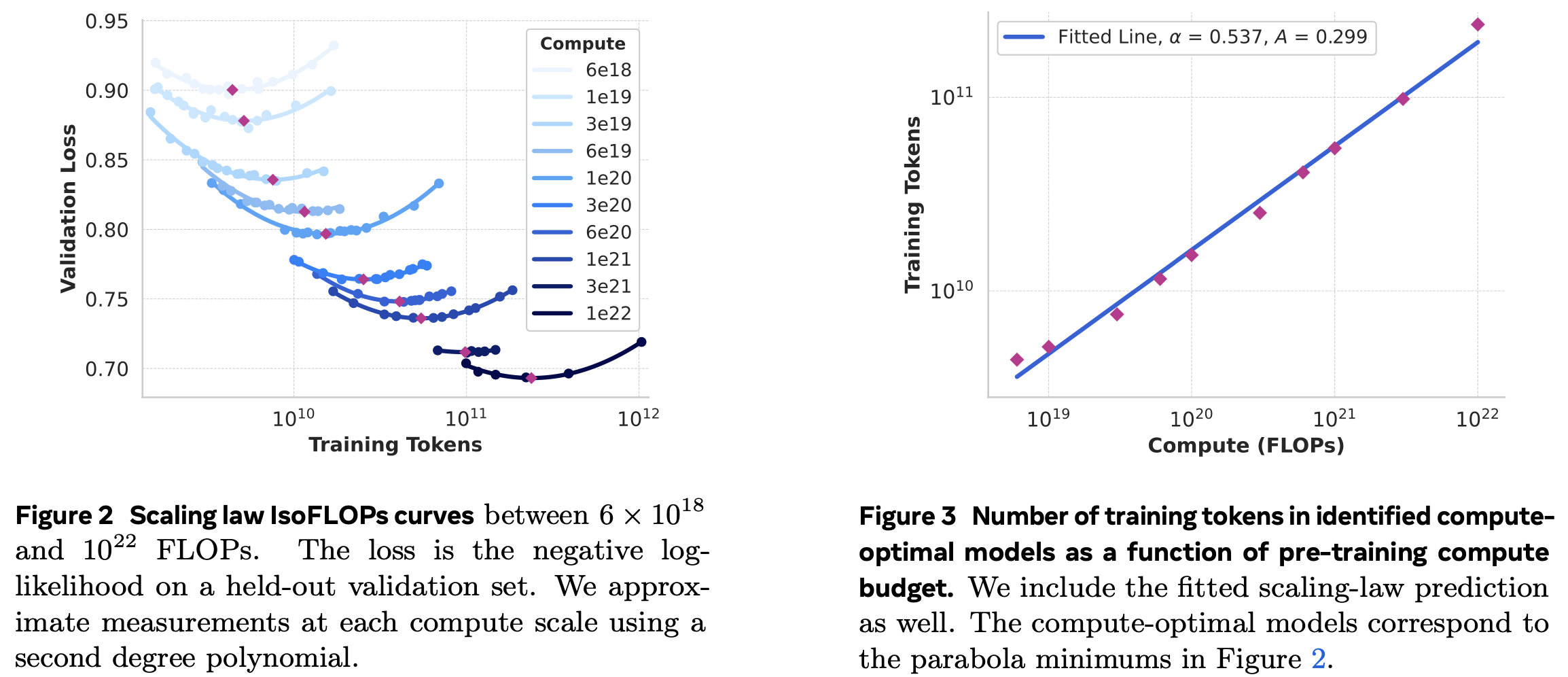
Llama 3 is “a herd of language models that natively support multi-linguality, coding, reasoning, and tool usage.” The models are made of 8B, 70B and 405B parameters and a context window of 128K tokens. Llama 3 405B uses an architecture with 126 layers, a token representation dimension of 16,384, and 128 attention heads. Llama 3 405B is trained on up to 16K H100 GPUs, via 4D parallelism (tensor, pipeline, context and data). The authors used scaling laws (Hoffmann et al., 2022;) to determine the optimal model size for our flagship model given our pre-training compute budget (section 3.2.1), where they establish a sigmoidal relation between the log-likelihood (figure 4):
The model architecture does not deviate from Llama 2, except that they:
- use grouped query attention with 8 key-value heads to improve inference speed and to reduce the size of key-value caches during decoding, and
- “use an attention mask that prevents self-attention between different documents within the same sequence as is important in continued pre-training on very long sequences”.
- vocabulary with 128K tokens: 100K from
tiktokenand 28k for better non-English support. - increase the RoPE base frequency hyperparameter to 500,000 to better support longer contexts.
Training is performed in two stages: pre-training via next-token prediction or captioning, and post-training where the model is “tuned to follow instructions, align with human preferences, and improve specific capabilities (for example, coding and reasoning).” The improvements were performed at 3 levels:
- at the data level, the authors improved quality, quantity, pre-processing and curation. The dataset includes “15T multilingual tokens, compared to 1.8T tokens for Llama 2.”
- At the scale level, the model increased its size almost \(50 \times\), reaching now \(3.8 \times 10^{25}\) FLOPS; and
- managing complexity, where they used a regular transformer with minor adaptations instead of a mixture of experts, and “a relatively simple post-training procedure based on supervised finetuning (SFT), rejection sampling (RS), and direct preference optimization (DPO), as opposed to more complex reinforcement learning algorithms.” (section 4)
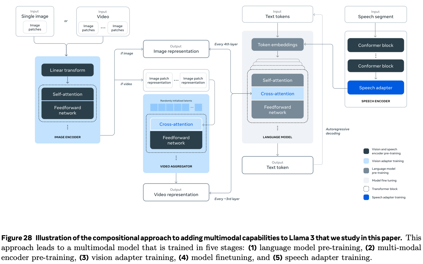
The authors also experiment adding image, video, and speech capabilities, by adding three additional stages:
- multi-modal encoder pre-training, where train and speech encoders are trained separately (sections 7 and 8). The image encoder is trained large amounts of image-text pairs, using self-supervised learning that “masks out parts of the speech inputs and tries to reconstruct the masked out parts via a discrete-token representation”.
- vision-adapter training, where the authors train an adapter on text-image pairs to align image representations with language representations. Then they train a video adapter on top of the image adapter on paired video-text data, to enable model to aggregate information across frames (section 7).
- Speech adapter training: a third adapter converts speech encodings into token representations.
The image encoder is a standard vision transformer trained to align images and text, the ViT-H/14 variant. They introduce cross-attention layers (Generalized Query Attention) between the visual token representations produced by the image encoder and the token representations produced by the language model, at every 4th layer.
Results (section 5) investigate the “performance of: (1) the pre-trained language model, (2) the post-trained language model, and (3) the safety characteristics of Llama 3”.
In section 6, they investigated two main techniques to make inference with the Llama 3 405B model efficient: (1) pipeline parallelism on 16 H100s with BF16 and (2) FP8 quantization. FP8 quantization is applied to most parameters and activations in feed-forward network but not to parameters of self-attention layers of the model. Similarly to Xiao et al 2024b they use dynamic scaling factors for better accuracy (with upper bound of 1200), and do not perform quantization in the first and last Transformer layers, and use row-wise quantization, computing scaling factors across rows for parameter and activation matrices.
2024 Universal Checkpointing: Efficient and Flexible Checkpointing for Large Scale Distributed Training, Microsoft DeepSpeed
According to the paper, the issue with state-of-the-art distributed checkpointing (model save/resume) is that it requires “static allocation of GPU resources at the beginning of training and lacks the capability to resume training with a different parallelism strategy and hardware configuration” and usually it is not possible to resume when hardware changes during the training process. To this extent, the paper proposes “Universal Checkpointing, a technique that enables efficient checkpoint creation while providing the flexibility of resuming on arbitrary parallelism strategy” and “ improved resilience to hardware failures through continued training on remaining healthy hardware, and reduced training time through opportunistic exploitation of elastic capacity”. This is achieved by writing in the universal checkpoint format, which allows “mapping parameter fragments into training ranks of arbitrary model-parallelism configuration”, and universal checkpoint language that allows for “converting distributed checkpoints into the universal checkpoint format”. The UCP file is a gathering of all distributed saves into a single file per variable type (optimizer state, parameters, etc).
2024 Domino: Eliminating Communication in LLM Training via Generic Tensor Slicing and Overlapping, Microsoft DeepSpeed
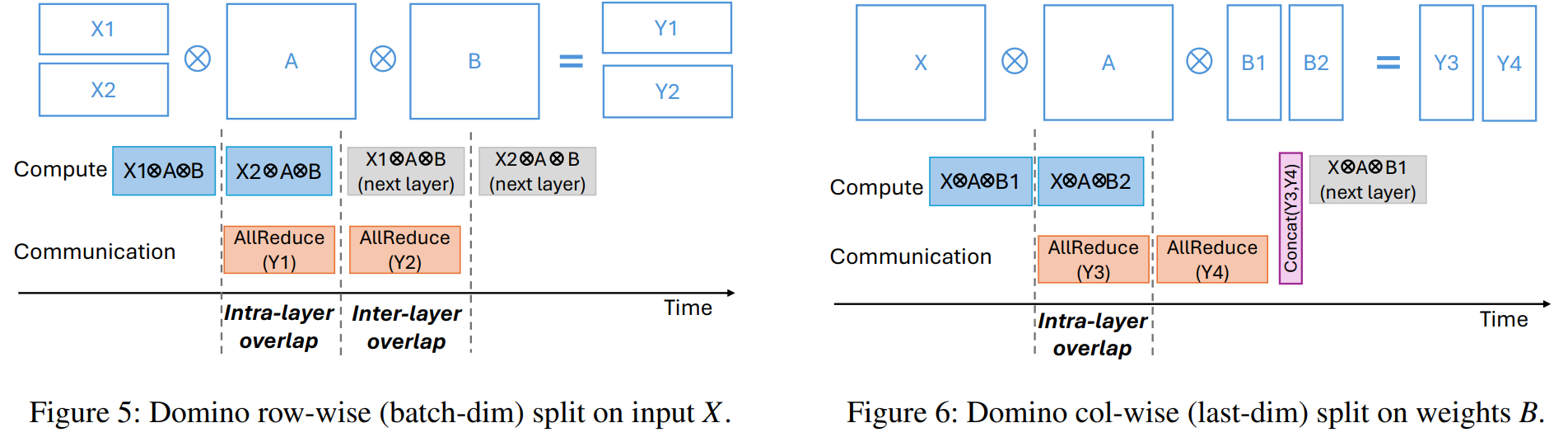
Domino “provides a generic scheme to hide communication behind computation” when training large LLMs where tensor parallelism (TP) is applied. “By breaking data dependency of a single batch training into smaller independent pieces, Domino pipelines these independent pieces training and provides generic strategy of fine-grained communication and computation overlapping. … comparing with Megatron-LM, Domino achieves up to 1.3x speedup for LLM training on Nvidia DGX-H100 GPUs”. The rationale for the paper is: current efforts to overlap computation and communication during TP are not enough, especially “in the cases where collective communication takes much longer than a single GeMM computation, most of the communication time still stands out as the major training overhead”. And “given that computation on the latest GPUs is becoming faster, communication overhead is more pronounced”. The paper proposes “Domino, a generic approach that breaks data dependency of transformer model training into pieces, and then pipelines these pieces training to overlap communication with computation …. Domino provides a much wider scope of computation and communication overlapping (e.g., AllReduce not only overlaps with a single GeMM, but also LayerNorm, DropOut, etc). … To hide TP communication behind computation, Domino provides extra and generic tensor partition in two dimensions on every GPU: row-wise split on inputs X and column-wise split on weights B on top of original TP model partitions. At high level, Domino generically breaks TP’s \(X \cdot A \cdot B\) into smaller compute units without data dependency. Then it pipelines these independent compute units with collective communication to achieve fine-grained computation and communication overlapping … we keep \(A\) untouched and do not conduct any tensor partitioning on \(A\). Therefore, we only conduct tensor slicing on input tensor \(X\) (section 3.2) and the second group of linear weights as \(B\) (section 3.3). We also provide a hybrid tensor partition strategy of both \(X\) and \(B\) (section 3.4). After these tensor slicing, Domino breaks \(X \cdot A \cdot B\) into pieces and removes data dependency. Then we enable computation-communication overlapping on these independent pieces to reduce communication overhead in TP.”
2023 Simplifying Transformer Blocks, ETH Zurich
A simpler transformer architecture that claims similar results to state-of-the-art autoregressive decoder-only and BERT encoder-only models, with a 16% faster training throughput, while using 15% fewer parameters.
![]()
2024 The Road Less Scheduled, Meta
“Existing learning rate schedules that do not require specification of the optimization stopping step T are greatly out-performed by learning rate schedules that depend on T.” The Schedule-Free approach is an optimization method that does not need the specification of T by removing the need of schedulers entirely. It requires no new hyper-parameters.
Backgroung: take the typical SGD optimization with step size \(γ\) in the form \(z_{t+1} = z_t − γ_{g_t}\), where \(g\) is the gradient at step \(t\). “Classical convergence theory suggests that the expected loss of this \(z\) sequence is suboptimal, and that the Polyak-Ruppert (PR) average \(x\) of the sequence should be returned instead” as \(x_{t+1} = (1 − c_{t+1}) x_t + c_{t+1} z_{t+1}\). If we use \(c_{t+1} = 1/(t+1)\), then \(x_t = \frac{1}{T} \sum_{t=1}^T z_t\). As an example, after 4 steps we have:
\[\begin{align*} x_1 = & z_1\\ x_2 = & \frac{1}{2} x_1 + \frac{1}{2} z_2, \\ x_3 = & \frac{2}{3} x_2 + \frac{1}{3} z_3, \\ x_4 = & \frac{3}{4} x_3 + \frac{1}{4} z_4, \\ x_5 = & \frac{4}{5} x_4 + \frac{1}{5} z_5, \\ \end{align*}\]However, “despite their theoretical optimality, PR averages give much worse results in practice than using the last-iterate of SGD”:

Recently, Zamani and Glineur (2023) and Defazio et al. (2023) showed that the exact worst-case optimal rates can be achieved via carefully chosen learning rate schedules alone, without the use of averaging. However, LR schedulers requise the definition of the stopping time T in advance. So the question of the paper is:
Do there exist iterate averaging approaches that match the empirical performance of learning rate schedules, without sacrificing theoretical guarantees?
This paper shows that it exists by introducing “a new approach to averaging that maintains the worst-case convergence rate theory of PR averaging, while matching and often exceeding the performance of schedule-based approaches”, demonstrated on 28 problems. Schedule-Free methods show strong performance, matching or out-performing heavily-tuned cosine schedules. The formulation of this Schedule-Free SGD is:
\[\begin{align*} y_t = \, & (1 − β) z_t + β x_t, \\ z_{t+1} = \, & z_t − γ∇f(y_t, ζ_t), \\ x_{t+1} = \, & (1 − c_{t+1}) x_t + c_{t+1} z_{t+1}, \\ \end{align*}\]where \(f(y_t, ζ_t)\) is the loss between model output and random variable \(ζ\), \(c_{t+1}\) is defined as before and \(z_1 = x_1\). “Note that with this weighting, the \(x\) sequence is just an online equal-weighted average of the \(z\) sequence. This method has a momentum parameter \(β\) that interpolates between Polyak-Ruppert averaging (\(β = 0\)) and Primal averaging (\(β = 1\)). Primal averaging is the same as PR except that gradient is evaluated at the averaged point \(x\), instead of \(z\) (see paper for definition), and “maintains the worst-case optimality of PR averaging but is generally considered to converge too slowly to be practical (Figure 2).”
The main point is: “The advantage of our interpolation is that we get the best of both worlds. We can achieve the fast convergence of Polyak-Ruppert averaging (since the \(z\) sequence moves much quicker than the \(x\) sequence), while still keeping some coupling between the returned sequence \(x\) and the gradient-evaluation locations \(y\), which increases stability (Figure 2). Values of β similar to standard momentum values \(β ≈ 0.9\) appear to work well in practice.”
2023 Training and inference of large language models using 8-bit floating point
The paper “presents a methodology to select the scalings for FP8 linear layers, based on dynamically updating per-tensor scales for the weights, gradients and activations.” The FP8 representation tested is the FP8E4 and FP8E5, for 4 and 5 bits of exponent, respectively. Despite the naming, intermediate computation is performed on 16 bits. The bias and scaling operations are applied to the exponent, not the final value. They tested two scaling techniques, AMAX (described before), or SCALE (keeping scale constant), and noticed there isn’t a major degradation. Results this fp8 to fp 16, but do not compare to bfloat16 because hardware was not available at the time. Algorithm in Figure 3. Note to self: I dont understand how so operations in float8 can be faster than half the executions in bfloat16 (because the workflow is so large); so it’s probably only faster than float16 because also requires a longer workflow with scaling (?).
2023 DeepSpeed ZeRO-Offload++: 6x Higher Training Throughput via Collaborative CPU/GPU Twin-Flow
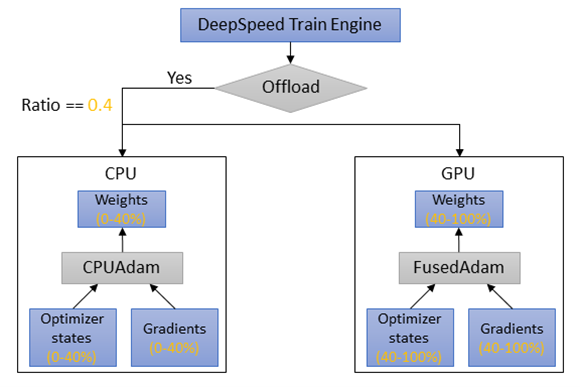
“System efficiency is still far from optimal when adopting ZeRO-Offload in some scenarios. Especially in the cases like small batch training, model that could not fit into GPU memory but not orders-of-magnitude bigger than GPU memory capacity, CPU offload not only introduce long end-to-end latency, but also underutilize GPU computation resources.” With that in mind, Zero-Offload++ introduces 3 fetures:
- Twin-Flow: instead having an all-or-nothing policy (ie offload all or none of) in the values to be offloaded, “Twin-Flow allows a portion of optimizer states to be held in CPU memory and the other portion of optimizer states remaining in GPU memory. When optimization step is triggered, both CPU and GPU can do parameter updates simultaneously.” The user can choose the percentage of ratio of parameters in CPU and GPU. “Therefore, with Twin-Flow, we can achieve decent GPU memory and core utilization rate, at the same time reduce training iteation time in optimizer offloading cases.”
- MemCpy reduction: details not available yet;
- CPUAdam optimization: details not available yet;
2023 DistFlashAttn: Distributed Memory-efficient Attention for Long-context LLMs Training (LightSeq), UC Berkeley et al.
DistFlashAttn extends FlashAttention from a single GPU to a distributed, sequence-parallel setting for training long-context LLMs. FlashAttention already turns attention’s quadratic peak memory into linear by computing it tile-by-tile with online softmax and never materializing the full score matrix. The split is by sequence (tokens), not by head or by feature dimension. Each GPU stores the Q, K, and V for its own token chunk only — full hidden dimension, all heads, just fewer rows. The challenge is doing this efficiently under causal attention, and the paper contributes three techniques
-
Token-level workload balancing: causal masking means a token only attends to its prefix, so a GPU holding early tokens has little work while one holding late tokens does quadratically more—a severe imbalance in naive sequence parallelism. DistFlashAttn rebalances this work across devices so no worker sits idle waiting for the heavily loaded ones.
-
Overlapping KV communication: like Ring Attention, K/V chunks are passed between GPUs so each device can attend to remote tokens, but DistFlashAttn overlaps that communication with the local attention computation, hiding the transfer latency behind useful work.
-
Rematerialization-aware gradient checkpointing: standard checkpointing recomputes a layer’s forward pass during the backward pass to save memory, but applied naively to FlashAttention it redundantly recomputes the attention—DistFlashAttn makes checkpointing aware of what FlashAttention already recomputes, avoiding the double work.
One framing difference to Ring Attention: Ring Attention is a fairly general sequence-parallel attention mechanism (works for inference and training, causal or not). DistFlashAttn is specifically tuned for causal, long-context LLM training — the load imbalance and the checkpointing interaction are both problems that only really bite in that setting.
Together these let it train 2–8× longer sequences and run faster than the alternatives of the time: 4.45–5.64× over Ring Self-Attention, 1.24–2.01× over Megatron-LM with FlashAttention, and 1.26–1.88× over Ring Attention and DeepSpeed-Ulysses, tested on Llama-7B at 32K–512K tokens. It solves the causal load-imbalance and checkpointing problems specific to the backward pass. It’s applied to training only, there’s no inference use case. DistFlashAttn is essentially Ring Attention plus three fixes for causal training: Causal load balancing (the biggest one); Communication/computation overlap; and 3. Rematerialization-aware gradient checkpointing.
2023 Chimera: An Analytical Optimizing Framework for Effective Compute-intensive Operators Fusion, Peking Univ., Shanghai AI Lab
Chimera (Zheng et al.) is a compiler framework that fuses chains of compute-intensive operators—like back-to-back GEMMs, or GEMM-then-softmax in attention—into single kernels to improve data locality. The motivation: as hardware compute throughput has outpaced memory bandwidth, even compute-heavy operators like GEMM and convolution end up memory-bound when run as a chain, because each operator writes its full output to memory only for the next to read it back. Existing ML compilers lacked both precise analysis and good optimization for these chains on different accelerators, so they left performance on the table. Chimera’s key idea is to break each operator into a series of computation blocks and then optimize at two levels. For inter-block optimization it uses an analytical model to pick the block execution order that minimizes data movement between blocks (so intermediate results stay in fast on-chip memory instead of round-tripping to DRAM); for intra-block optimization it generates an efficient hardware-specific “micro-kernel.”
Examples from the paper:
- The GEMM→GEMM chain
C = A×BandE = C×Dwhere a tile ofCwill be immediately used to computeE, without fully instantiatingC.- if we had assinged to each GPU block a tile of
E, there would be a lot of contention and the need to introduce atomic. Instead, here, they assign to each GPU block: a full row ofAandE, it produces and immeidately iterates tiles ofC, and iterates all columns ofBandD.
- if we had assinged to each GPU block a tile of
- Batch GEMM chain (attention).
Q×Kᵀ → softmax → ×V— two batch GEMMs with a softmax in the middle. - Convolution chain (CNNs). A
3×3 conv → ReLU → 1×1 conv → ReLUfused into one kernel — common in ResNet-style nets, memory-bound at certain input shapes.
Because it relies on an analytical cost model rather than exhaustive auto-tuning, Chimera produces fused kernels in minutes instead of the hours search-based compilers like Ansor need. The three pieces each matter—on average the cost model contributes ~2.37×, fusion ~1.89×, and the micro-kernel ~1.61×. End to end, fusing GEMM-with-GEMM chains gives 2.62× over PyTorch, 4.78× over Relay, 1.40× over Ansor, and 3.28× over oneDNN, plus ~1.62× over PyTorch for GEMM-chain-plus-softmax. The work is hardware-portable, targeting both CPUs and Tensor Core GPUs.
2023 ZeRO++: Extremely Efficient Collective Communication for Giant Model Training, Microsoft
DeepSpeed ZeRO’s compute throughput is limited by the high communication cost from gathering weights in forward pass, backward pass, and averaging gradients. This is mostly prominent on clusters with low-bandwidth, and at very small batch sizes per GPU.
Background, communication pipeline: “Assume the model size as 𝑀. During the forward pass, ZeRO conducts an all-gather operation to collect all the parameters (𝑀) needed to train for all model layers. In the backward pass, ZeRO re-collects parameters (𝑀) with all-gather first, then each GPU can compute local gradients. After that, ZeRO operates reducescatter function to aggregate and redistribute gradients (𝑀) across accelerators. In total, ZeRO has a total communication volume of 3𝑀, spreads evenly across 2 all-gather and 1 reduce-scatter.”
The paper introduces three communication reduction techniques, packed as ZeRO++:
- Quantized Weight Communication for ZeRO (qwZ): perform block quantization of the forward all-gather, converting weights from FP16 (2 bytes) to INT8 (1 byte). The main improvement is to replace the typical quantization algorithm (multiplying all parameters by a scalar), by a quantization per block (ie per parameter subset) that includes multiplication by a factor and shifting values by another factor;
- Hierarchical Weight Partition for ZeRO (hpZ): data remapping that trades-off communication for more memory and reduces communication overhead of all-gather on weights during backward. Instead of having weights distributed across GPUs, we maintain a full copy on each machine, allowing us to replace the expensive cross-machine all-gather on weights with a faster intra-machine all-gather.
- Quantized Gradient Communication for ZeRO (qgZ): replaces the gradients reduce-scatter collective, by doing (1) block-based quantization of gradients to
INT4during communication to reduce the communication size, and recovering the full precision before the reduction operator to preserve training accuracy. Having a fully block-based quantization approach like in (1) was also considered but led to high precision loss and a high error propagation across layers during backpropagation.
The results sections claims that ZeRO++ yields a communication reduction of 4x compared to ZeRO-3, leading to up to 2.16x higher compute throughput on 384 GPUs.

2023 QLoRA: Efficient Finetuning of Quantized LLMs, Washington Uni
“An efficient finetuning approach that reduces memory usage enough to finetune a 65B parameter model on a single 48GB GPU while preserving full 16-bit finetuning task performance. QLORA backpropagates gradients through a frozen, 4-bit quantized pretrained language model into Low Rank Adapters (LoRA). QLORA introduces multiple innovations designed to reduce memory use without sacrificing performance: (1) 4-bit NormalFloat, an information theoretically optimal quantization data type for normally distributed data that yields better empirical results than 4-bit Integers and 4-bit Floats. (2) Double Quantization, a method that quantizes the quantization constants, saving an average of about 0.37 bits per parameter (approximately 3 GB for a 65B model). (3) Paged Optimizers, using NVIDIA unified memory to avoid the gradient checkpointing memory spikes that occur when processing a mini-batch with a long sequence length. We use QLORA to finetune more than 1,000 models, [and] results show that QLoRA finetuning on a small high-quality dataset leads to state-of-the-art results, even when using smaller models than the previous SoTA”. Notes to self:
- 4-bit NormalFloat Quantization rounds values to the nearest bin (in a 4-bit representation) where each bin is a normal distribution quantile. It’s an expensive procedure, so they use fast quantile approximation algorithms such as SRAM. It also yields high errors for outliers.
2023 Better speech synthesis through scaling (TorToise), James Bekter
The paper describes a way to apply ML for generating images to the speech synthesis. This result is TorToise, an expressive, multi-voice text-to-speech system. So far, TTS models were hard to train eficiently due to high sampling rate, unavailability of large datasets, or encoder-decoder challenges.
Background: most modern text-to-speech systems operate on speech data that is encoded as a MEL spectrogram. Because of this, most efforts focus on the high-quality decoding of MEL spectrograms back into audio waveforms, a.k.a. a vocoder or a MEL inverter. The author dives in the state-of-the-art autoregressive transformers and DDPMs models:
- DALL-E, a transformer model with a (quadratic complexity) full-sequence self-attention, that showed how an autoregressive decoder can be applied to text-toimage generation. The author believes that the “VQVAE decoder used by DALL-E is principally responsible for the blurry incoherence exhibited by most of it’s samples”.
- DALL-E also introduced the process of re-ranking, that samples from the autoregressive model and picks the best output for downstream use. Re-ranking requires a a strong discriminator to tell good from bad text/image pairings. CLIP was used for this purpose.
- Denoising diffusion probabilistic models (DDPMs) generate crisp high quality images, and are effective on using low-quality signals to reconstruct the high-dimensional space where those signals derived from. However, DDPMs rely on fixed output shapes, know beforehand. Thus, they “ cannot learn to convert text into audio signals because they cannot solve the implicit alignment problem between text and audio”. Also, DDPMs must be sampled from over multiple iterations, leading to high compute cost and latency.
With that in mind: TorToise works by joining autoregressive decoders and DDPMs: “the autoregressive model will be used to convert a sequence of text tokens to a sequence of tokens representing the output space (in our case, speech tokens). The DDPM will then be used to decode these tokens into a high quality representation of speech.” In practice, for Text-To-Speech, we train the following neural networks:
- An auto-regressive model on text tokens that yields the probability of each audio token;
- A contrastive model that ranks outputs of the autoregressive decoder. DALL-E uses CLIP (for images), but TorToise uses Contrastive Language-Voice Pretrained Transformer (CLVP, for TTS).
- A DDPM to convert speech tokens back into speech spectrograms;
The inputs of the auto-regressive and DDPM models include (or are conditioned to) an additional speech conditioning input, which is one or more audio clips (MEL spectograms) of the same speaker as the target. This allows the model to learn “infer vocal characteristics like tone and prosody” are desired in the target output audio. Finally, they apply the TorToise trick: the DDPM is first trained on converting discrete speech codes into MEL spectrograms, and then fine-tuned on the latent space of the AR model outputs instead of the speech codes. “The logic here is that the AR latent space is far more semantically rich than discrete tokens. By fine-tuning on this latent space, we improve the efficiency of the downstream diffusion model”

2023 Neural Codec Language Models are Zero-Shot Text to Speech Synthesizers (VALL-E), OpenAI
The paper introduces a pipeline for text-to-speech translation (TTS), based on a neural codec language model (VALL-E) using discrete codes (encode/decode embeddings) derived from an off-the-shelf neural audio codec model (Encoded, Défossez et al., 2022). This mode treats TTS as a conditional language modeling task rather than continuous signal regression as in previous work. In practice, contrarily to e.g. AudioLM, a generative audio-to-audio / speech-to-speech model that predicts future audio from input audio, VALL-E is a TTS mode that takes as input a fixed-size text representation and the audio of the first 3 seconds of the text, and tries to predict the future audio that matches the remaining of the input text. VALL-E uses an audio codec code as intermediate representation and language model as objective, contrary to previous models using mel spectrogram as intermediate representaion and continuous signal regression as objective. VALL-E is trained with the LibriLight dataset, consisting of 60K hours of English speech with over 7000 unique speakers. This dataset is audio-only, so the authors employ a speech recognition model to generate the (text) transcriptions.
Background, quantization, tokenizer and encoding: audio is typically stored as a sequence of 16-bit integer values, therefore a generative model is required to output \(2^{16}\) = 65536 probabilities per timestep to synthesize the raw audio. Added to the high output size, its long sequence length makes it more intractable for audio synthesis. Therefore, speech quantization is required to compress integer values and sequence length. Common methods are \(\mu\)-law, vector quantization (HuBERT, vq-wav2vec), k-means/self-supervised method, etc. As audio tokenizer, VALL-E uses a pre-trained neural audio codec model, EnCodec, a convolutional encoder-decoder model, whose input and output are both 24 kHz audio across variable bitrates. The encoder produces embeddings at 75 Hz for input waveforms at 24 kHz, which is a 320-fold reduction in the sampling rate. Each embedding is modeled by residual vector quantization (RVQ), with eight hierarchy quantizers with 1024 entries each as shown in Figure 2.
Model architecture: formally speaking, \(Encodec(y) = C^{T \times 8}\), where \(C\) represents the two-dimensional acoustic code matrix (the 8-channel audio embeddings), and \(T\) is the downsample utterance length. Each row in \(C\) represents the eight codes for a given time frame. After quantization, the neural codec decoder is able to reconstruct the waveform, i.e. \(Decodec(C) ≈ \hat{y}\). Given an accoustic prompt matrix \(\hat{C}^{T \times 8}\), the optimization objective of the TTS model is \(max\, p(C \mid x, \hat{C})\), where \(x\) is the corresponding phoneme transcription. I.e. the model learns to extract the content and speaker information from the phoneme sequence and the acoustic prompt, respectively.
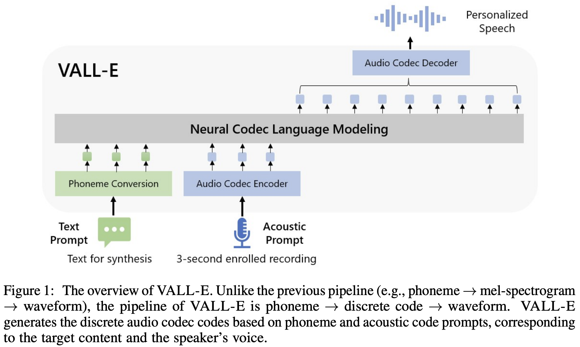
There are two models, that refer to the two inference steps:
- an auto-regressive (AR) model, a transformer decoder-only architecture, conditioned on the phoneme (text) and accoustic prompt (3-second audio), that gives the discrete tokens of the audio from the first quantizer (Formula 1).
- a non auto-regressive (NAR), a transformer decoder will full mask, that regressively predicts the remaining 7 quantizers from the first one (Formula 2).

Note to self: for the use case of synthethising audio in a different language, i.e. that differs from the 3-sec input language and text, see VALL-E X.
2023 High-Fidelity Audio Compression with Improved RVQGAN, Descript Inc.
An audio encoder-decoder that supposedly beats Meta’s encodec. Achieved by combining advances in high-fidelity audio generation with better vector quantization techniques from the image domain, along with improved adversarial and reconstruction losses. Methods:
- to account for periodicity in audio inputs, they adopted the snake activation function for frequency \(\alpha\) as \(snake(x) = x + \frac{1}{α} sin^2 (αx)\).
- vanilla VQ-VAEs struggle from low codebook usage due to poor initialization, leading to a significant portion of the codebook being unused. This leads to to poor reconstruction quality. To address this issue, they use two techniques: (1) factorized codes that decouples code lookup and code embedding, by performing code lookup in a low-dimensional space (section 3.2) and (2) L2-normalization of the encoded and codebook vectors converts euclidean distance to cosine similarity, which is helpful for stability and quality.
- state-of-the-art applying quantizer dropout degrades the audio reconstruction quality at full bandwidth. To overcome it, they instead apply quantizer dropout to each input example with some probability \(p=0.5\).
- an improved STFT discriminator at multiple time-scales, that works better in practice and leads to improved phase modeling, compared to Encodec and Soundstream.
- for frequency domain reconstruction loss, they use a mel-reconstruction loss to improve stability, fidelity and convergence speed; and multi-scale spectral losses to encourage modeling of frequencies in multiple time-scales. For adversarial loss, they use HingeGAN. For codebook learning, they use commitment losses with stop-gradients from the original VQ-VAE formulation. All these losses are weighted to sum up to the final loss.
2023 Llama 2: Open Foundation and Fine-Tuned Chat Model, Meta
LLama 2 is a collection of pretrained and fine-tuned large language models (LLMs) ranging in scale from 7 billion to 70 billion parameters. Llama 2-Chat is a finetuned LLM optimized for dialogue use cases. The models outperform open-source chat models, and based on human evaluations for helpfulness and safety, it outperforms open-source models and appear to be on par with closed-source models (although may not be a suitable substitute). Results on safety human evaluation for Llama 2-Chat are presented in Figure 3. The train dataset is only publicly available sources, which does not include data from Meta’s products or services, or sources that may include users’ personal information. Table 2 presents the GPU compute hours, power consumption and carbon emissions of each model
The pretraining setting and model architecture are adopted from Llama 1, i.e. bytepair encoding (BPE), pre-normalization via RMSNorm, SwiGLU activations, rotary positional embeddings, AdamW optimizer, cosine learning rate scheduler. However, the primary architectural differences from Llama 1 include increased context length and grouped-query attention (GQA).
The finetuning was performed with supervised fine-tuning (Section 3.1), initial and iterative reward modeling (Section 3.2.2) and RLHF (Section 3.2.3). As drawback of RLHF, “initial RLHF models tended to forget the initial instruction after a few turns of dialogue (Figure 9, below, left). To address these limitations, we propose Ghost Attention (GAtt), a very simple method inspired by Context Distillation (Bai et al., 2022b) that hacks the fine-tuning data to help the attention focus in a multi-stage process”. In Gatt, ghost tokens are introduced at specific intervals or positions, and do not represent actual data but serve as intermediate “proxies” to summarize information across groups of tokens. (Figure 9, below, right).

2023 LLaMA: Open and Efficient Foundation Language Models, Meta
LLaMa is a collection of Large Language Models (LLM) with 7B to 65B parameters trained in public datasets, with performance superior to GPT-3 and comparable with Chinchilla-70B and PaLM-540B. Training is inspired by the Chinchilla scaling laws. The datasets used for the pre-training data are presented in Table 1, with training hyperparameters in Table 2. String are tokenized using the bytepair encoding (BPE) algorithm, with circa 1.4T tokens after tokenization.
The models architecture is made of several improvements over the original Transformer:
- Pre-normalization [GPT3]: training stability is improved with RMSNorm normalization at the input of each transformer sub-layer, instead of output.
- SwiGLU activation function [PaLM]: ReLU activation is replaced with SwiGLU to improve performance, with a dimension of \(\frac{2}{3} 4d\) instead of \(4d\) as in PaLM.
- Rotary Embeddings [GPTNeo]: positional embeddings are replaced by rotary positional embeddings (RoPE) at each layer of the output.
- Optimization performed with AdamW optimizer with \(β_1 = 0.9\), \(β2 = 0.95\) and \(eps = 10^{−5}\).
- Cosine learning rate schedule with a warmup of \(2000\) steps, a weight decay of \(0.1\), a gradient clipping of \(1.0\) and a final learning of \(10%\) of the initial value.
- Efficient causal multi-Head attention achieved by not storing the attention weights and not computing the key/query scores that are masked due to the causal nature of the language modeling task.
- Activation checkpointing was implemented to reduce memory. Yet it required manually implementing the Pytorch backward propagation function for the Transformer (insted of PyTorch autograd). This also required model and sequence parallelism (why?).
- Overlap of the computation of activations and the communication between GPUs over the network, to reduce latency.
2023 Sparks of Artificial General Intelligence: Experiments with an early version of GPT-4, Microsoft
A summary paper reporting early results of the experiments with GPT-4 when it was still in active development by OpenAI. The authors “demonstrate that, beyond its mastery of language, GPT-4 can solve novel and difficult tasks that span mathematics, coding, vision, medicine, law, psychology and more, without needing any special prompting. Moreover, in all of these tasks, GPT-4’s performance is strikingly close to human-level performance”. The bulk of the paper contains dozens of examples that compare GPT-4 and Chat-GPT and demonstrate that GPU-4 surpasses ChatGPT in performance, in code generation, audio generation (output as musical notes), drawings (SVG, TIKZ), and mathematical resolutions (LaTeX). As weaknesses, besides the regular hallucinations it was also observed:
- Incapacity of planning correctly, when planning is not a linear path.
- Occasional arithmetic mistakes on long expressions (without tool use), highlighting limits in exact computation.
- Trained on past information only, without real-time/temporal awareness.
- lack of rigorous algorithms e.g.
What is the 11th letter of "abacadab"? … the 11th letter is "b." - Analogical reasoning can reproduce social stereotypes present in training data.
But these can be overcome by including external APIs on training and making them in the query e.g.:
2023 Retentive Network: A Successor to Transformer for Large Language Models, Microsoft and Tsinghua University
(note: a simpler summary video of RetNet can be found here)
RetNet is a multi-scale retention mechanism to substitute multi-head attention in Transformers, which has three computation paradigms:
- parallel framework, for training parallelism that utilizes GPU devices fully.
- recurrent framework for low-cost \(O(1)\) inference, which improves decoding throughput (8.4x improvement over Transformer), latency (15.6x), and GPU memory (3.4x) without sacrificing performance, on Figure 1.
- a chunkwise recurrent representation that can perform efficient long-sequence modeling with linear complexity, where each chunk is encoded parallelly while recurrently summarizing the chunks. It allows encoding each local block for computation speed while recurrently encoding the global blocks to save GPU memory
Retentive network (RetNet) is a stack of \(L\) identical blocks, which follows a similar layout (i.e., residual connection, and pre-LayerNorm) as in Transformer. Each RetNet block contains two modules: a multi-scale retention (MSR) module, and a feed-forward network (FFN) module. The MSR module calls the tokens in a sequence in an auto-regressive manner. The input vector is first created as \(X_0\) in the shape of sequence length by hidden domain size. Then we calculate contextualized vector representations \(X_n\) for each layer of the RetNet. Retention heads can be represented in two alternative ways:
- in the parallel representation, where \(Retention(X) = Q K\intercal \dot D)V\) similar to the transformer but with an extra matrix \(D\) (Eq. 5). This is befenicial for parallel training.
- in the recurrent representation, it is written as a recurrent neural net (RNN) which is beneficial for inference, and \(Retention(X_n)=Q_n S_n\) where \(S_n\) depends on the previous term \(S_{n-1}\).
- a hybrid form combining the previous two representations is also possible to accelerate training on large sequences. Input sequence is divided into chunks. Within each chunk, the computation is performed in the parallel representation. Cross-chunk information is passed in the recurrent representation.
Finally, the model uses \(h = d_{model}/d\) retention heads in each layer, where \(d\) is the head dimension. The heads use different parameter matrices \(W_Q, W_K, W_V \in \mathbb{R}^{d \times d}\) and scalar \(γ\) per head. The overall architecture for a given layer \(l\) of the RetNet is then \(Y_l = MSR(LayerNorm(X_l)) + X_l\) and \(X_{l+1} = FFN(LN(Y_l)) + Y_l\), ie similar to a regular transformer but replacing the attention by a retention head.

2023 RoFormer: Enhanced Transformer with Rotary Position Embedding (Rotary Embedding, RoPe)
Traditional positional encoding methods, like sinusoidal or learned embeddings, struggle to generalize well to long sequences because they either: (1) Use absolute positions that are fixed and cannot model relative relationships effectively. (2) Lack a mechanism to extrapolate beyond the sequence lengths seen during training. Rotary embeddings address these issues by encoding relative positional information directly into the attention mechanism, improving efficiency and generalization. “RoPE encodes the absolute position with a rotation matrix and meanwhile incorporates the explicit relative position dependency in self-attention formulation”.
Rotary embeddings modify the query (𝑄) and key (K) embeddings in self-attention. They do this by applying rotations to the embeddings based on the positions of tokens in the sequence.
\[R(x) = \begin{bmatrix} \cos\theta & -\sin\theta \\ \sin\theta & \cos\theta \end{bmatrix} \cdot \begin{bmatrix} x_1 \\ x_2 \end{bmatrix}\]The rotation angle \(𝜃_𝑝\) for position \(p\) is determined as \(𝜃_𝑝 = p \, w\), where \(w\) is a frequency determined by the dimensionality and scaling factors. Important bit: \(x_1\) and \(x_2\) are the input \(x\) expressed in the 2D coordinates. To handle a \(d\)-dimensional input, we split \(x\) into pairs of dimensions \([ (x_1, x_2), \, (x_3, x_4), \, \dots, \, (x_{d-1}, x_d)]\), apply the 2D rotation matrix to each pair, and then concatenate the results to reconstruct the rotated vector. If \(x\) has an odd dimensionality \(d\), the extra dimension is often left unrotated.
2023 Operator Fusion in XLA: Analysis and Evaluation, UToronto
Kernel fusion is the most significant optimization operation in XLA. This paper details XLA and key compiler passes of XLA’s source code. It also presents the speedup that kernel fusion can deliver, and what low-level effects it has on hardware.
2023 LongNet: Scaling Transformers to 1,000,000,000 Tokens, Microsoft and Xi’an Jiaotong University
LongNet is a Transformer variant that can scale the sequence length up to 1B tokens, and without sacrificing the performance on shorter sequences. This overcomes current limitations of attention size in regular transformers, that requires a tradeoff between computational complexity and the model expressivity. The main trick is based on the dilated attention, which is similar to strided attention but with exponentially increasing strides (e.g., attending to tokens at distances 1, 2, 4, 8, etc.).
2023 FlashAttention-2: Faster Attention with Better Parallelism and Work Partitioning
“FlashAttention is still not nearly as fast as optimized matrix-multiply (GEMM) operations, reaching only 25-40% of the theoretical maximum FLOPs/s. We observe that the inefficiency is due to suboptimal work partitioning between different thread blocks and warps on the GPU, causing either low-occupancy or unnecessary shared memory reads/writes. We propose FlashAttention-2, with better work partitioning to address these issues. In particular, we (1) tweak the algorithm to reduce the number of non-matmul FLOPs (2) parallelize the attention computation, even for a single head, across different thread blocks to increase occupancy, and (3) within each thread block, distribute the work between warps to reduce communication through shared memory. These yield around 2× speedup compared to FlashAttention, reaching 50-73% of the theoretical maximum FLOPs/s on A100 and getting close to the efficiency of GEMM operations. We empirically validate that when used end-to-end to train GPT-style models, FlashAttention-2 reaches training speed of up to 225 TFLOPs/s per A100 GPU (72% model FLOPs utilization).”
2023 Flow Matching for Generative Modeling
Flow Matching is a a simulation-free approach for training CNFs (Continuous Normalizing Flows) that is compatible with a general family of Gaussian probability paths for transforming between noise and data samples, as required by the reverse process in diffusion models. “Furthermore, Flow Matching opens the door to training CNFs with other, non-diffusion probability paths. An instance of particular interest is using Optimal Transport (OT) displacement interpolation to define the conditional probability paths. These paths are more efficient than diffusion paths, provide faster training and sampling, and result in better generalization”. See a good explanation in this Cambridge ML group post</summary> .
2022 Titans: Learning to Memorize at Test Time, Google Research
A model that utilizes recurrent logic and attention, like mamba. From the abstract: “We present a new neural long-term memory module that learns to memorize historical context and helps an attention to attend to the current context while utilizing long past information. We show that this neural memory has the advantage of a fast parallelizable training while maintaining a fast inference. From a memory perspective, we argue that attention due to its limited context but accurate dependency modeling performs as a short-term memory, while neural memory due to its ability to memorize the data, acts as a long-term, more persistent, memory.”
2022 Flow Straight and Fast: Learning to Generate and Transfer Data with Rectified Flow
Rectified flows aim at reducing the number of steps when transitioning between two distributions. This is important for e.g. diffusion models where we perform inference by performing \(T\) sampling steps and we want to do it in less steps, by finding a flow between interleaved steps. The rectified flow is an ODE model that transport distribution \(π_0\) to \(π_1\) by following straight line paths as much as possible. The straight paths are preferred both theoretically because it is the shortest path between two end points, and computationally because it can be exactly simulated without time discretization
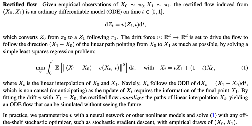
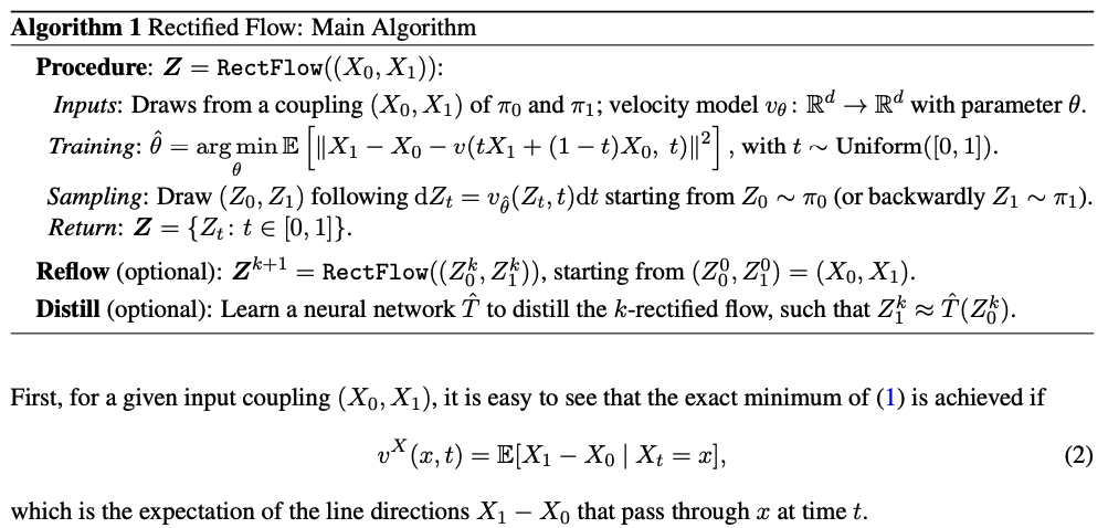
2022 Tensor Programs V: Tuning Large Neural Networks via Zero-Shot Hyperparameter Transfer (\(\mu\)Transfer), Microsoft
Maximal Update Parametrization (muP) showed that many optimal hyper-parameters remain constant as the mode size changes: “When (layer) width is large, every activation vector has roughly iid coordinates, at any time during training. Using Tensor Programs, we can recursively calculate such coordinate distributions, and consequently understand how the neural network function evolves”.
With that in mind, here, here they propose a hyper-parameter tuning paradigm called muTransfer: “parametrize the target model in muP, tune the HP indirectly on a smaller model, and zero-shot transfer them to the full-sized model”.
![]()
Figure 1: Training loss against learning rate on Transformers of varying \(d_{model}\) trained with Adam. Conventionally and in contrast with our technique, different widths do not share the same optimal hyperparameter; wider networks do not always perform better than narrower ones; in fact they underperform the same-width networks in our technique even after tuning learning rate (see dashed line).
Hyperparameters That Can Be µTransferred, Not µTransferred, or µTransferred Across (Depth), with a few caveats discussed in Section 6.1. * means empirically validated only on Transformers, while all others additionally have theoretical justification.
- µTransferable: optimization related (learning rate, momentum, Adam beta, LR schedule, etc), init (per-layer init variance), parameter multipliers (multiplicative constants after weight/biases, etc), etc
- Not µTransferable: regularization (dropout, weight decay, etc)
- µTransferred Across (Depth): width, depth, batch size, training time, seq length
2022 Self-Attention Does Not Need (O(n^2)) Memory
Rabe & Staats formalize the idea that self-attention can be computed without storing the full (n \times n) attention matrix by using a streaming / online computation of the softmax-normalized attention. This is a conceptual ancestor of several practical kernels: it gives the mathematical justification for computing attention in blocks while maintaining numerical stability and correctness.
Why it still matters in modern systems papers:
- It provides a clean argument for why “don’t materialize (QK^\top)” is not just an approximation—it can be exact.
- It underpins many attention kernels that trade memory for compute and enable long-context attention to be feasible.
2022 DeepSpeed-Inference: Enabling Efficient Inference of Transformer Models at Unprecedented Scale (SC 2022)
DeepSpeed-Inference is a systems paper about getting Transformer inference to scale in practice: kernel fusion (to reduce memory traffic and launch overhead), parallelism strategies, and memory optimizations that allow very large models to run efficiently.
In the context of fusion-heavy related work:
- DeepSpeed-Inference aggressively fuses compute (Transformer kernels, projections, etc.) and optimizes the inference runtime, but generally keeps communication as NCCL collectives outside of those kernels.
- This makes it a useful baseline class: it shows what you can get from strong kernel engineering and runtime scheduling without changing the underlying communication model.
Results / takeaways: the paper demonstrates that systematic kernel/runtime optimizations can unlock large-scale inference and high throughput, and it established many techniques that later LLM serving stacks built on.
2022 DeepSpeed-MoE: Advancing Mixture-of-Experts Inference and Training to Power Next-Generation AI Scale (ICML 2022)
DeepSpeed-MoE is an influential MoE system that focuses on making expert models train and run efficiently by addressing the MoE-specific bottlenecks: token routing, all-to-all communication, and balancing compute/communication across experts. It includes runtime techniques to overlap communication with local work and reduce overhead in the MoE pipeline.
How it compares to later MoE system lines (MegaScale-*):
- DeepSpeed-MoE provides a general MoE framework and many practical optimizations, but later production-scale systems often introduce more specialized parallelism strategies and communication libraries to handle extreme scale.
- DeepSpeed-MoE is also representative of approaches that keep collectives “standard” (NCCL-style), whereas newer kernel-level work explores in-kernel collectives and fine-grained overlap.
Results / takeaways: the paper demonstrates that MoE can scale effectively with careful engineering, and it helped popularize MoE as a practical path to scaling model capacity without proportional compute.
2022 DeepSpeed Inference: Enabling Efficient Inference of Transformer Models at Unprecedented Scale, Microsoft DeepSpeed
Inference kernels must therefore achieve high memory bandwidth utilization and high compute utilization at small batch sizes, whereas training kernels simply need to achieve high compute utilization at much larger batch sizes. This makes developing inference kernels quite challenging. DeepSpeed Inference consists of two components:
- DeepSpeed Transformer: DeepSpeed Inference can automatically scale a dense transformer model to multiple devices by partitioning transformer operators across multiple devices while also adding appropriate communication operations needed across GPUs. Under the hood, it leverages the single GPU kernels to maximize per GPU memory bandwidth utilization, while using NCCL all-reduce collectives to perform the necessary across GPU communication. This allows DeepSpeed Inference to achieve excellent aggregate memory bandwidth utilization across several GPUs with a node. However, tensor slicing can not be scaled efficiently beyond a single node due to significant communication overhead. Thus to further scale to multi-node systems, DeepSpeed Inference uses pipeline parallelism. DeepSpeed Transformer includes three transformer modules:
- a single GPU transformer kernels for minimizing latency and maximizing throughput via memory-bandwidthcentric fusion schedules and GeMM kernels (Sec. III). This is described below.
- A many-GPU dense transformer inference system that combines tensor-parallelism to minimize latency with inference optimized pipeline parallelism schedules and memory optimizations to maximize throughput (Sec. IV). The model and pipeline parallelism techniques are then applied on top of the single GPU kernels.
- A massive-GPU sparse (MoE) model inference system that combines: i) expert, data, and tensor parallelism, ii) novel communication optimizations and iii) sparse kernel optimizations to scale sparse inference on trillions of parameters across hundreds of GPUs (Sec. V). Expert parallelism is also introduced, where all-to-all can happen within just the subset of devices that share the same tensor-slicing rank, since the data across tensor-parallel ranks are replicated. The sparse tensor representation in the gating function and sparse einsum operators introduce a significant latency overhead, optimized with kernel fusion.
- ZeRO-Inference that leverages CPU, NVMe and GPU memory along with GPU compute to make massive model inference accessible with limited resources (Sec. VI). An important design decision is how to apportion GPU memory among model weights, inference inputs, and intermediate results. One approach is to pin as much of the model weights as possible into GPU memory, and fetch the remainder (from DRAM or NVMe) when needed for computation. The big downside is that allow for a small batch size. ZeRO-Inference adopts a different approach that pins the model weights either in DRAM (if large enough) or NVMe, and streams each layer into GPU memory for computation when needed.
The single GPU transformer kernels introduce two techniques:
- Deep-Fusion to reduce kernel-invocation and data-movement overheads by fusing multiple kernels beyond element-wise operation. The rationale is: on GPU, if a data produced by a thread-block is consumed by a different one, a global memory synchronization is needed which invokes a new kernel. To avoid the need for a global synchronization, Deep-Fusion tiles the computation-space along dimensions of the iteration space which incur no cross-tile data-dependencies and executes them in parallel across different thread-blocks. The dimensions of the computation-space which does contain data dependencies are not tiled, and instead processed by the same thread-block. After this tiling, two operators can be fused using DeepFusion if each tile of the second operator depends on exactly one output tile of the first operator. Deep-Fusion can fuse not only element-wise operations but also reductions, data transpositions, and GeMMs as long as there are no cross-tile dependencies.
- a Custom GeMM implementation designed to be fusable with Deep-Fusion while achieving maximum memory bandwidth utilization. “We first tile the computation along the output dimension. That allows us to implement GeMM using a single kernel by keeping the reduction within a tile” Then, with the aforementioned tiling strategy, each warp in a thread block is responsible for producing a partially reduced result for a tile of outputs and a final reduction is needed across all the warps within the thread block. To avoid having to reduce the partial results in shared memory, we perform a single data-layout transpose in shared memory such that partial results of the same output element are contiguous in memory, and can be reduced by a single warp using cooperative-group collectives directly in registers. Finally, we also transpose the weight matrix during initialization such that M rows for each column are contiguous in memory. We fuse the operations inside a transformer layer at four main regions: 1) the QKV GeMM and input layer-norm, 2) transposition plus attention, 3) postattention layer-norm and intermediate GeMM, and 4) bias and residual addition.
2022 DyLoRA: Parameter Efficient Tuning of Pre-trained Models using Dynamic Search-Free Low-Rank Adaptation
LoRA blocks “suffer from two major problems: first, the size of these blocks is fixed and cannot be modified after training (for example, if we need to change the rank of LoRA blocks, then we need to re-train them from scratch); second, optimizing their rank requires an exhaustive search and effort”. Dynamic LoRA (DyLoRA) addresses these two problems. “DyLoRA method trains LoRA blocks for a range of ranks instead of a single rank by sorting the representation learned by the adapter module at different ranks during training”. How does it work:
- In each LoRA module, we have an up-projection (\(W_{up} ∈ R^{m×r}\)) and a down-projection matrix (\(W_{dw} ∈ R^{r×d}\)). Let’s assume that we would like to train the LoRA module to operate in the range of \(r ∈\) Range \([r_{min}, r_{max}]\) where \(r_{min}\) and \(r_{max}\) are hyper-parameters.
- At each training step, we sample \(b\) (a value between ranks \(r_{min}\) and \(r_{max}\)), and truncate \(W_{dw}\) and \(W_{up}\) to include only \(b\) columns/rows, accordingly. The truncated matrices are represented as \(W_{dw↓b}\) and \(W_{up↓b}\), and they’re the ones used in this training step: \(h = W_0x + \frac{α}{b} W_{up↓b} W_{dw↓b} x\).
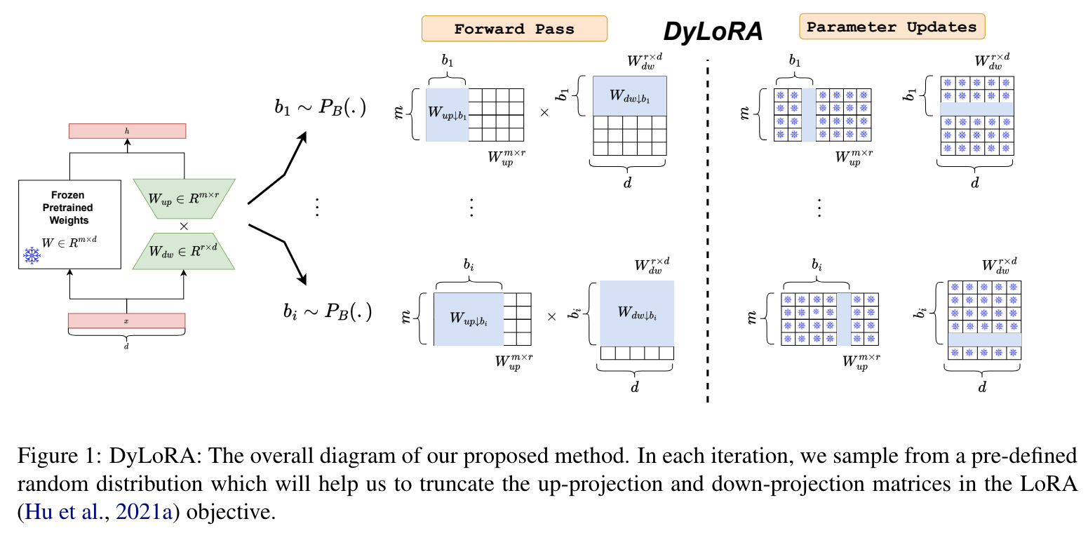
2022 Efficiently Scaling Transformer Inference, Google
The paper focuses on efficient generative inference of Transformer models with large deep models, with tight latency targets and long sequence lengths. It claims its methods surpass the efficiency of NVIDIA’s FasterTransformer. It is highly foccused on 3D-torus network layouts.
Section 3.1 provides an analysis of collective communication. Section 3.2 analyzes parallelism in the FeedForward module. Notation used: \(BLE_{xyz}\) means that the last dimension \(E\) of a tensor of logical shape \(BLE\) is split into \(X × Y × Z\), ie the per-chip tensor is of shape \([B, L, E/(X × Y × Z)]\) (omitted axis are replicated). \(F\) is the input size of the feed forward layer. It compares data splitting a la Megatron (1D weight-stationaly layout, section 3.2.1) where the partition layout for weights is \(EF_{xyz}\) and \(F_{xyz}E\), i.e. partitioned in to \(X × Y × Z = n_{chips}\); with a 2D weight-stationary layout along both the E and F axes (section 3.2.2), where shards are square, compute cost is the same but communication is more efficient and scalable (particularly on more than 16 chips). Section 2.3.3 describes the XYZweight-gathered approach, where “the output of each per-chip matrix multiplication must then be aggregated between chips to be used as input to the subsequent operations”, however “for very large batch sizes, it is best to keep the activations fully stationary between sequential matrix multiplications, requiring that we fully transfer the weights between all chips”.
Related to attention layers (section 3.3), “Multihead attention can be parallelized in essentially the same ways as a feedforward layer”. The attention Keys and Values (aka the “KV cache”) incur significant memory capacity and bandwidth costs. Improving with multi-query attention reduces the size of the KV cache tensors by a factor of \(n_{heads}\) and the time spent loading them in memory, but “removes an axis otherwise used for parallelism, so the KV cache and related computations need to be partitioned differently” in order to “minimize the memory time of repeatedly loading the KV cache that dominates the inference cost. … The most similar partitioning layout for multiquery attention (shown in Figure 4(b)) treats the KV cache the same as in multihead attention. Even though the key and value tensors are shared across all heads, they must be replicated on each chip and the memory cost savings of multiquery attention are lost”. Instead the paper proposes “ a partitioning strategy for the multiquery attention where the Q, K, and V matrices are partitioned over the batch \(B\) dimension into \(n_{chips}\) partitions”. This reduces the cost of loading the KV cache per chip by a factor of \(n_{chips}\) but incurs additional communication cost of resharding the input activation tensors. “With the proposed partitioning layout, multiquery attention enables using larger batch sizes and sequence lengths, thereby increasing throughput in addition to the latency reduction from reduced memory time”.
![]()
Section 3.4 details the gains of using GPT-J’s approach to compute attention heads and feed forward in parallel, also applied to PaLM. For comparison, the standard formulation of the transformer block is \(y = x + MLP(LayerNorm(x + Attention(LayerNorm(x)))\), whereas the parallel formulation is: \(y = x + MLP(LayerNorm(x)) + Attention(LayerNorm(x))\). Using the parallel formulation has only one layernorm per layer instead of two, which reduces latency at small batch sizes. Also, some matrices can be fused which results in larger matrix multiplications that run more efficiently on accelerators. Finally, it removes one of the two all-reduce operations in each layer.
Finally, section 3.5 discusses low-level optimization (overlapping communication and computation, etc), and section 3.6 discusses int8 quantization.
2022 Random-LTD: Random and Layerwise Token Dropping Brings Efficient Training for Large-scale Transformers, Microsoft
Random-LTD (random and layerwise token dropping method) is a method to reduce the training costs of very large transformer models, which skips the computation of a subset of the input tokens at all middle layers (exclude first and last layers). Tokens are dropped in a purely random matther, thus Random-LTD requires no scoring or manual design.
Other alternatives of token dropping are:
- attention score related metrics, where compute cost for LTD is too high since the metric has to be calculated for every layer); and
- loss-/frequency-based metrics, where accumulated loss or frequency is used and this accumulated metric would not be changed within the same iteration (forward pass), and this makes the dropped token to be the same for different layers, making the token dependency not be captured by the MHA of middle layers.
To that extent, Random-LTD uses purely random dropping of tokens at every layer. To reduce the gradient variance introduced by random-LTD, for better training, the authors monotonically increase the kept sentence length throughout training, with a linear schedule. This method is called the Monotonic Sequence Length Growth (MSLG).
Related to the learning rate, not that: random-LTD reduces the effective batch size of middle layers at the initial warmup phase, and MSLG does not reach the full length until > 2/3 of training iterations for large compute saving. Therefore, the small learning rate during warmup cannot provide efficient training “dynamics” for Random-LTD. In practice, it is necessary to increase the warmup iterations and slow down the LR decay. So the paper also introduces the LayerToken learning rate (appendix C), wich scales the learning rate based on the sum of consumed tokens of each layer. The point of LayerToken is to reduce the tuning effort for Random-LTD.
The results compare Random-LRD with the baseline, on GPT3 models with 350M and 1.3B parameters, and a dataset of up to 300B tokens. Here, Random-LTD shows similar evaluation losses as the baseline with 1/3 less LayerToken consumption. However, an important claim is that “reiterate that the LayerToken consumption saving ratio cannot directly transfer to GPU wall-clock training time saving ratio due to the implementation/hardware”. Compared with a BERT and ViT model, similar results are shown. When compared with TokenBypass (a different technique that skips middle layers tokens), Random-LTD shows better train and validation perplexity. Also, MLSG also shows better perplexity than a constant-drop rate (table 6.4).
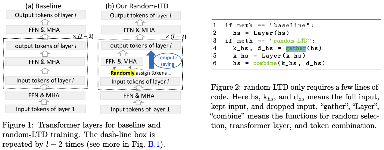
2022 The Stability-Efficiency Dilemma: Investigating Sequence Length Warmup for Training GPT Models, Microsoft
This paper investigates and demonstrates the importance of sequence length in GPT models. The paper presents a set of experiments on a GPT2 model on public datasets to study the stability-efficiency dilemma: “increasing the batch sizes and learning rates (commonly used for faster training) leads to better training efficiency but can also result in training instability, leading to poor generalization accuracy or failed runs”. The paper results that there is a strong correlation between training instability and extreme values of gradient variance and long sequence lengths contribute to these extreme gradient variance values, especially at the beginning of the training (and this could be a source of traininig instability).
The paper presents the “Sequence Length Warmup (SLW) method (which starts training with short sequences and gradually increases the length) that aims to solve the training stability-efficiency dilemma by avoiding extreme gradient variance values. This method can be understood as a type of curriculum learning (CL), which presents easier/simpler examples earlier during training and gradually increases the sample difficulties. However here, the work aims to achieve both efficient convergence and better stability by enabling stable training with more aggressive hyperparameters, instead of keeping them constant as in the traditional CL.
Results show improved stability, an increase of 4x in batch size, and 8x in learning rage on a 117M and 1.5B parameter GPT2 model. On a GPT3 model, it demonstrates 8x larger batch size and 40x larger learning rate, retaining 99% of one-shot accuracy using 10x less data and 17x less time.
2022 FlashAttention: Fast and Memory-Efficient Exact Attention with IO-Awareness
Transformers are slow and memory-hungry on long sequences, since the time and memory complexity of self-attention are quadratic in sequence length. The authors “ argue that a missing principle is making attention algorithms IOaware—accounting for reads and writes between levels of GPU memory”. To overcome it, Flash Attention improves the attention mechanism with one that uses tiling to reduce the number of memory reads/writes between GPU high bandwidth memory (HBM) and GPU on-chip SRAM. In practice, it tiles the square attention matrix into partial computations that can be computed on the block memory (on-chip SRAM) instead of the global memory (DRAM?). It also trains Transformers faster than existing baselines (15% on bert models and 3x on GPT-2).

FlashAttention is the canonical example of algorithmic fusion in attention: it avoids materializing the full (QK^\top) (and often avoids materializing large intermediate softmax buffers) by using a numerically stable streaming formulation. Instead of computing attention as “GEMM → softmax → GEMM” with large intermediate tensors in HBM, it tiles the computation so that data is reused from SRAM/shared memory.
How it differs from “FFN fusion + in-kernel communication” work:
- FlashAttention is primarily about IO-aware tiling of attention and a streaming softmax trick, not about overlapping distributed communication.
- It shows that fusion can change the algorithmic memory complexity (and not just launch overhead), which is why it became such a cornerstone kernel.
Results / takeaways: the original FlashAttention work reports large practical gains (commonly multiple× speedups in attention throughput and significant memory savings), and it established the template that later fusion work often emulates: fuse stages, tile aggressively, and never write big intermediates to HBM if you can stream them instead.
2022 High Fidelity Neural Audio Compression (Encodec), Meta AI
Encoded is a neural network model for a real-time, high-fidelity, audio codec. It consists in a streaming encoder-decoder architecture with quantized latent space trained in an end-to-end fashion. For faster and simpler training, they use a single multiscale spectrogram that efficiently reduces artifacts and produce high-quality samples. Two main problems arise in lossy neural compression of audio. The first one is overfitting to a subset of audio simples, and it was overcome by using (1) a large and diverse dataset and (2) discriminator networks that serve as perceptual loss. The second problem is compressing efficiently, both in compute time and in size, solved by using residual vector quantization of the neural encoder floating-point output. The authors claim that “designing end-to-end neural compression models is a set of intertwined choices, among which at least the encoder-decoder architecture, the quantization method, and the perceptual loss play key parts”. To that extent, audio quality evaluations (MUSHRA) consist in having humans listen to, compare, and rate excerpts of speech or music compressed with competitive codecs.
Background and model: An audio signal of duration d can be represented by a sequence \(x ∈ [−1, 1]^{C_a × T}\) with \(C_a\) the number of audio channels, \(T = d · f_{sr}\) the number of audio samples at a given sample rate \(f_{sr}\). The EnCodec model is composed of three main components:
- an encoder network \(E\) that inputs an audio extract and outputs a latent representation \(z\). It’s simply a stack of 1D convolutions and pooling blocks, followed by a two-layer LSTM for sequence modelling, and a final 1D convolution with \(D\) output channels.
- a quantization layer \(Q\) produces a compressed representation \(z_q\), using vector quantization. They use Residual Vector Quantization (RVQ, Zeghidour et al. 2021) to quantize the output of the encoder. As background, general Vector Quantization consists in projecting an input vector onto the closest entry in a codebook of a given size. In this case, RVQ refines this process by computing the residual after quantization, and further quantizing it using a second codebook, and so forth.
- a decoder network \(G\) that reconstructs the time-domain signal, \(\hat{x}\), from the compressed latent representation \(z_q\). The decoder’s architecture is the inverse of the encoder, using transposed convolutions instead of strided convolutions.
There are two variants of the model, targetted for the low-latency streamable setup, or a high fidelity non-streamable usage.

The train objective minimizer a linear combination of the following loss products:
- reconstruction loss, comprised of a time and a frequency domain loss term, to minimize the L1 distance between the target and compressed audio over the time domain, i.e. \(l_t(x, \hat{x}) = \| x − \hat{x} \|_1\). For the frequency domain loss \(l_f\) (Note: type here, this \(l_s\) in the picture above, as in spectogram loss), they use an averaged sum of the L1 and L2 losses between the elements of the input and output mel-spectograms.
- discriminative loss, a perceptual loss term based on a multi-scale STFT-based (MS-STFT) discriminator, as in Figure 2. In practice, the decoder acts as a generator in a adversarial network and Encodec includes a discriminator module (in orange), with an adversarial loss for the generator as \(l_g(\hat{x}) = \frac{1}{K} \sum_k max (0, 1 − Dk(\hat{x}))\), where \(K\) is the number of discriminators. They add a similar additionally matching loss for the generator, \(l_{feat} (x, \hat{x})\), in Formula 2 (PS: where is this in Figure 1?). The discriminators are trained with the adversarial loss \(l_d(x, \hat{x}) = \frac{1}{K} \sum_{k-1}^K max (0, 1 − D_k(x)) + max(0, 1 + D_k(\hat{x}))\), where \(K\) is the number of discriminators.
- VQ commitment loss. To support Multi-bandwith learning, at 24 kHz, the model is trained to support the bandwidths 1.5, 3, 6, 12, and 24 kbps by selecting the appropriate number of codebooks to keep in the RVQ step (section 3.2). At 48 kHz, it’s trained to support 3, 6, 12 and 24 kbps. They add a commitment loss \(l_w\) between the output of the encoder, and its quantized value, with no gradient being computed for the quantized value. For each residual step \(c\), where \(C\) is the bandwidth: \(l_w = \sum_{c=1}^C \| z_c - q_c (z_c) \|_2\), where \(q_c(z_c)\) the nearest entry in the corresponding codebook.
The authors also claim that “We introduce a loss balancer in order to stabilize training, in particular the varying scale of the gradients coming from the discriminators” and “We additionally train a small Transformer based language model (Vaswani et al., 2017) with the objective of keeping faster than real time end-to-end compression/decompression on a single CPU core.” (Section 3.3) that I have skipped.
2022 DeepNet: Scaling Transformers to 1,000 Layers
This paper introduces a normalization function (DeepNorm) to modify the residual connection in Transformer, accompanyed with theoretically derived initialization, in order to stabilize extremely deep Transformers.
- Background: previous work had sown that better initialization methods improve the stability of the training of Transformer.
- DeepNorm works by introducing a new normalization function at residual connections, which has theoretical justification of bounding the model update by a constant.
- “The proposed method combines the best of two worlds, i.e., good performance of Post-LN and stable training of Pre-LN (picture above), making DeepNorm a preferred alternative.”.
- Figure 2 shows the
deepnorm(the normalization layer function),deepnorm_init(the weights initialization) and constants.
2022 Contrastive Deep Supervision, Tsinghua University, Intel Corporation, and Xi’an Jiaotong
From the abstract: “the traditional training method only supervises the neural network at its last layer and propagates the supervision layer-by-layer, which leads to hardship in optimizing the intermediate layers. Recently, deep supervision has been proposed to add auxiliary classifiers to the intermediate layers of deep neural networks. By optimizing these auxiliary classifiers with the supervised task loss, the supervision can be applied to the shallow layers directly. However, deep supervision conflicts with the well-known observation that the shallow layers learn low-level features instead of task-biased high-level semantic features. To address this issue, this paper proposes a novel training framework named Contrastive Deep Supervision, which supervises the intermediate layers with augmentation-based contrastive learning”. The rationale is that contrastive learning can provide better supervision for intermediate layers than the supervised task loss. Contrastive learning “regards two augmentations from the same image as a positive pair and different images as negative pairs. During training, the neural network is trained to minimize the distance of a positive pair while maximizing the distance of a negative pair. As a result, the network can learn the invariance to various data augmentation, such as Color Jitter and Random Gray Scale”. Contrastive Deep Supervision starts from those advancements, and optimizes the intermediate layers with contrastive learning instead of traditional supervised learning.

2022 Robust Speech Recognition via Large-Scale Weak Supervision (Whisper), OpenAI
Whisper is an automatic speech recognition (ASR) system, that performs several tasks on a Speech-to-text setup. It is trained on 680K hours of multilingual and multitask supervised data collected from the web. I.e. it’s a weakly supervised dataset. The authors “show that the use of such a large and diverse dataset leads to improved robustness to accents, background noise and technical language.
The Whisper architecture (section 2.2) is an encoder-decoder Transformer. Input audio is split into 30-second chunks, converted into a log-Mel spectrogram, and then passed into an encoder. A decoder is trained to predict the corresponding text caption, intermixed with special tokens that direct the single model to perform tasks such as language identification, phrase-level timestamps, multilingual speech transcription, and to-English speech translation.” Audio is re-sampled to 16,000 Hz, and an 80-channel logmagnitude Mel spectrogram representation is computed on 25-millisecond windows with a stride of 10 milliseconds. Whisper uses the same Byte-Pair Encoding text tokenizer as in GPT2 for english-only models and refit the vocabulary for other languages.
2022 Emergent Abilities of Large Language Models, Google Research & Stanford
The paper discusses instead the phenomenon of emergent abilities of large language models. An ability is emergent if it is not present in smaller models but is present in larger models, and not extrapolated from scaling laws. Phase transition is the scale at which such abilities are exposed. Scale in this context may represent different compute budgets, data quality or other factors - the paper foccuses not on ideal training but on the discussion of such phenomena. As a disclaimer, “model scale is not the singular factor for unlocking an emergent ability” and “the science of training large language models progresses, certain abilities may be unlocked for smaller models with new architectures, higher-quality data, or improved training procedures”.
The first analysis of emergent abilities focuses the prompting paradigm, where outcome is emergent when a model has random performance until a certain scale, after which performance increases to well-above random. This was analysed on 8 different models:
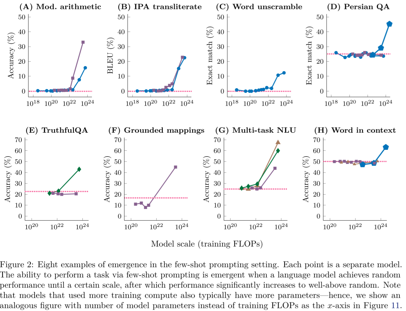
A similar analysis with augmented prompting exposes the emergent property as related to when the model output starts having a positive effect (e.g. being able to do arithmetic only after a certain scale). A multi-step reasoning by providing a chain-of-thoughts as a sequence of intermediate steps was also analysed, and claimed to be exposed only after \(10^{23}\) FLOPS or approx. 100B parameters. Such scale is also required for intruction following tasks (ie new tasks without prior few-shots exemplars, and only by reading a set of instructions). Program execution tasks require \(9 x 10^{19}\) FLOPS or 40M parameters (for a 8-digit addition) or larger. For model calibration (the ability of a model responding as True of False (or the correctness probability) to which questions they’ll be able to predict correctly) requires \(3*10^{23}\) FLOPS or 52B parameters. It is summarized as:

2022 Rethinking Attention with Performers, Google, Cambridge, DeepMind and Alan Turing Institute
From the abstract: Performers are “Transformer architectures which can estimate regular (softmax) full-rank-attention Transformers with provable accuracy, but using only linear (as opposed to quadratic) space and time complexity, without relying on any priors such as sparsity or low-rankness. To approximate softmax attention kernels, Performers use a novel Fast Attention Via positive Orthogonal Random features approach (FAVOR+)”.
A clearer explanation can be found on this google research post:
Bidirectional attention, where there’s no notion of past and future: by decouplin matrices \(Q′\) and \(K′\) used in lower rank decomposition of \(A\) and conducting matrix multiplications in the order indicated by dashed-boxes, we obtain a linear attention mechanism, never explicitly constructing \(A\) or its approximation:

Left: Standard attention module computation, where the final desired result is computed by performing a matrix multiplication with the attention matrix \(A\) and value tensor \(V\). Right: By decoupling matrices \(Q′\) and \(K′\) used in lower rank decomposition of \(A\) and conducting matrix multiplications in the order indicated by dashed-boxes, we obtain a linear attention mechanism, never explicitly constructing \(A\) or its approximation.
Unidirectional (causal) attention, where tokens do not attend to other tokens appearing later in the sequence: the previous approach is modified to use prefix-sum computations, which only store running totals of matrix computations rather than storing an explicit lower-triangular regular attention matrix.

Left: Standard unidirectional attention requires masking the attention matrix to obtain its lower-triangular part. Right: Unbiased approximation on the LHS can be obtained via a prefix-sum mechanism, where the prefix-sum of the outer-products of random feature maps for keys and value vectors is built on the fly and left-multiplied by query random feature vector to obtain the new row in the resulting matrix.
2022 Training Compute-Optimal Large Language Models, arXiv
Heavily related to HPC’s performance modelling applied to large language models. The authors revisit the question “Given a fixed FLOPs budget, how should one trade-off model size and the number of training tokens?” to which they present three approaches: (1) fix model sizes and vary number of training tokens; (2) vary model sizes for 9 different FLOP counts; (3) fit a parametric loss function to the values retrived from the 2 approaches. Estimates were collected from a total of 400 runs.
The main conclusion is that current large language models are under-performing as they only scaled the model size and not the data size. For compute-optimal training, the model size and number of training tokens should be scalled equally. This hypothesis is demonstrated with a “compute-optimal” model Chinchilla, with the same “compute budget” as Gopher (70B parameters) and 4× more more data. Chinchilla outperforms Gopher (280B), GPT-3 (175B), Jurassic-1 (178B), and Megatron-Turing NLG (530B) on several evaluation tasks.
To be compute optimal (in terms of accuracy vs energy cost), Kaplan et al. (2020) claims that models should not be trained to their lowest possible loss, and for a 10× increase in computational budget, the model should increase by 5.5× and the training tokens by 1.8x. In this paper, the authors defend that model size and training tokens should be scaled in equal proportions.
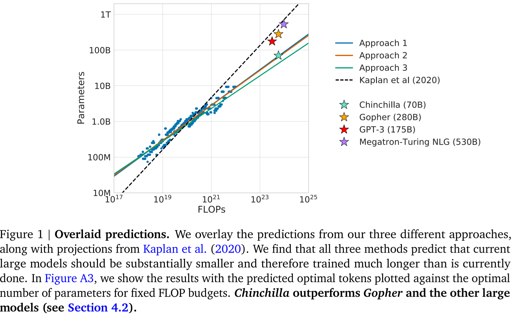
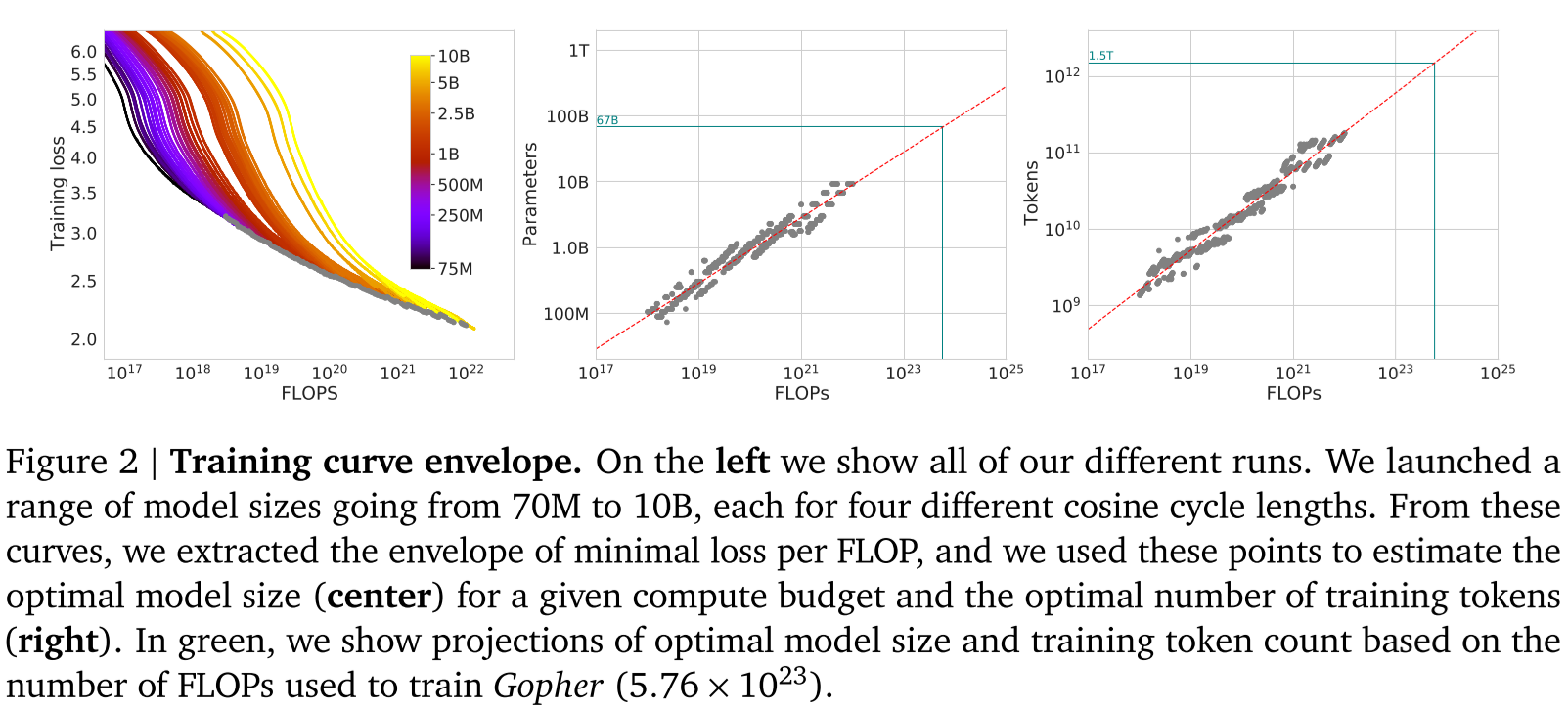
2021 Breaking the Computation and Communication Abstraction Barrier in Distributed Machine Learning Workloads
Abstract: the paper presents CoCoNet “with a DSL (Domain Specific Language) to express a program with both computation and communication. CoCoNeT contains several machine learning aware transformations to optimize a program and a compiler to generate high performance kernels. Providing both computation and communication as first class constructs allows users to work on a high-level abstraction and apply powerful optimizations, such as fusion or overlapping of communication and computation. CoCoNeT enables us to optimize data-, model-and pipeline-parallel workloads in large language models with only a few lines of code. “
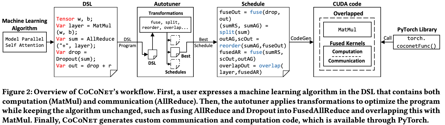
2021 LoRA: Low-Rank Adaptation of Large Language Models, Microsoft
Low-Rank Adaptation (LoRA) is a technique used to efficiently fine-tune large machine learning models by injecting trainable low-rank parameter updates into the model’s layers. It is particularly useful for adapting pre-trained models to new tasks or domains without retraining the entire model, which is computationally expensive and requires large storage resources.
LoRA focuses on decomposing parameter updates into low-rank matrices, drastically reducing the number of trainable parameters while maintaining the model’s expressive power.
A small, trainable low-rank matrix \(Δ𝑊\) is added to the original weight matrix \(𝑊\). The final output is \(W′=W+ΔW\). Instead of directly learning \(Δ𝑊\), it is factorized as \(ΔW=AB^⊤\) where \(A\) and \(B\) are low-rank matrices.
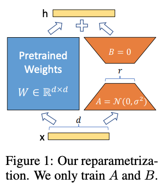
2021 Learning Transferable Visual Models From Natural Language Supervision (CLIP), OpenAI
Motivation: state-of-the-art vision systems are trained on a fixed predetermined set of objects (labels). Additional labeled data is needed to specify any other visual concept. However, “the development of text-to-text as a standardized input-output interface has enabled taskagnostic architectures to zero-shot transfer to downstream datasets, removing the need for specialized output heads or dataset specific customization”. A critical insight is that it is possible to leverage natural language as a flexible prediction space to enable generalization and transfer – ie train a text model, and then specialize it on a non-textual task. In practice, natural language is able to express, and therefore supervise, a much wider set of visual concepts through its generality. Learning from natural language also has an important advantage over most unsupervised or self-supervised learning approaches in that it doesn’t “just” learn a representation but also connects that representation to language which enables flexible zero-shot transfer.
With that in mind, this paper introduces a neural network called CLIP (Contrastive Language–Image Pre-training) which efficiently learns visual concepts from natural language supervision. By design, the network can be instructed in natural language to perform a great variety of classification benchmarks, without directly optimizing for the benchmark’s performance, similar to the “zero-shot” capabilities. CLIP models can then be applied to nearly arbitrary visual classification tasks. Thus, the main keypoint is: by not directly optimizing the model for the benchmark, we show that it becomes much more representative.
In practice, CLIP pre-trains an image encoder and a text encoder to predict which images were paired with which texts in our dataset. The dataset is an abundantly available source of supervision: 400 million pairs of text and respective images found across 500K queries from the internet. For the image encoder, the authors consider 5 differently-sized ResNet50 (with improvements such as attention pooling similar to a QKV attention), and 3 Vision Transformers. The text encoder is a transformer with masked self-attention, with Byte-Pair encoding with a 49152 vocab size. The max sequence length was capped at 76 (section 2.4).
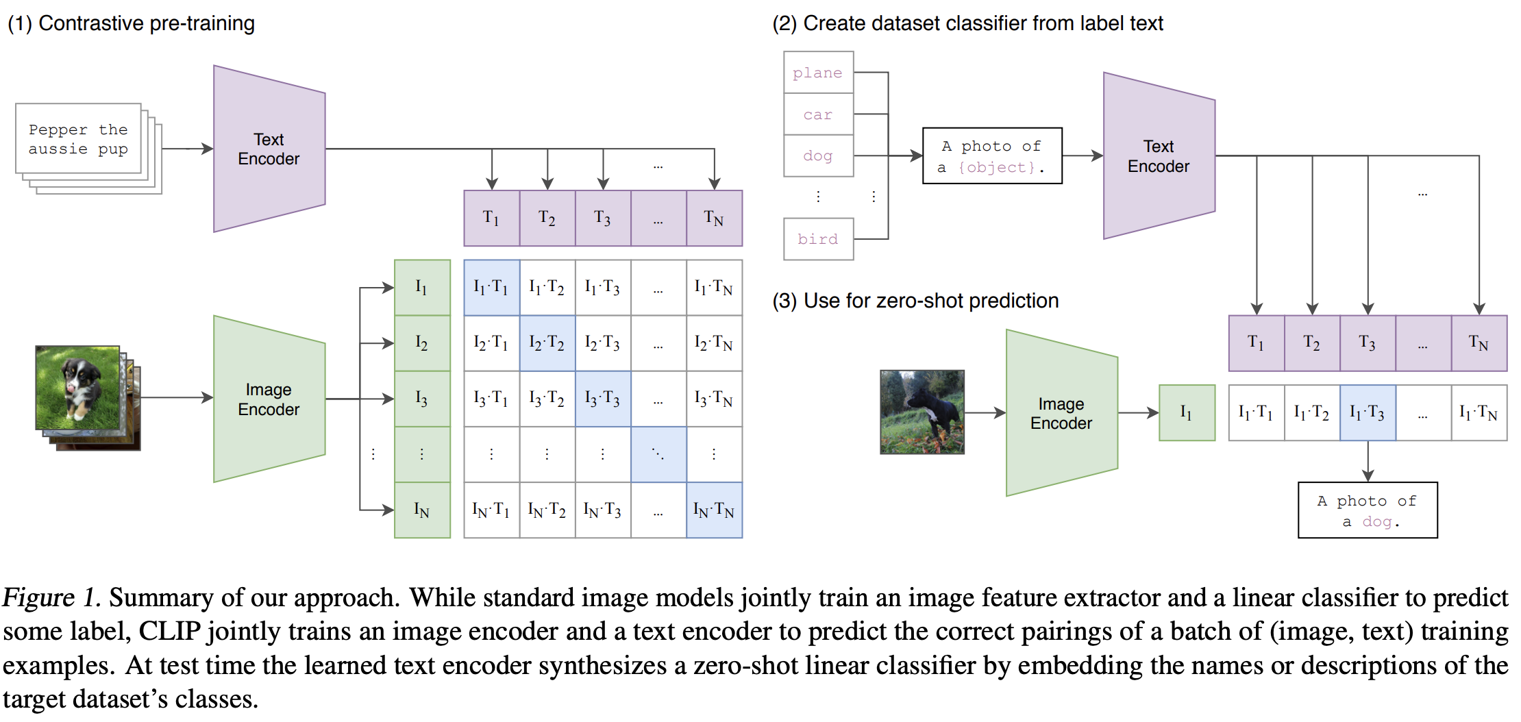
The pipeline for contrastive pre-training (1) is the following:
- we pass an image through the image encoder (ViT or ResNet). Each image \(i\) is pictured as \(I_i\) above.
- we pass the text through the text decoder (transformer). Each text \(i\) is pictured as \(T_i\), analogously.
- the diagonal of the \(I_i T_j\) matrix is the correct image/text labels (in blue).
- We use contrastive learning and train related text and images to be maximally close, and unrelated to be minimally close. In practice, we maximize the inner product of
Nlabels that go together (full row and full column of the diagonal cells) and minimize the inner product of theN^2-Nlabels that dont go together (full row and full column of the non-diagonals). We then interpret the product as a logit and then use the softmax on both directions to get the loss (ie it’s a symmetric loss from text and image perspective).- in practice, in contrastive learning, “the cosine similarity (i.e. cosine of the angle) of these embeddings is then calculated, scaled by a temperature parameter τ , and normalized into a probability distribution via a softmax”. See figure 3 for source code. scores.
- In practice, for each image input e.g. \(I_3\), we get the classification distributions \(I_3 T_1\), \(I_3 T_2\), \ldots, \(I_3 T_N\).
As you can tell from section (1) in the picture, minibatch size N is critical. As the minibatch approximates the entire dataset, the representations are more detailed. And the computation of the matrix \(I_i T_j\) increases (quadratically?).
During inference, in (2), we create a dataset by taking a set of labels and adding a prompt to all labels e.g. A photo of a {label}. We then put them through the text encoder, and that is our target set.
Then, to perform zero-shot prediction (3), we take an image, pass it through the image decoder, and get the classification distribution of that image over the prompted labels, from where we pick the top label - in the picture A photo of a dog.
The main point is: there was zero training needed on the entire task, the image and test datasets can be entirely different, which is a fundamental difference to regular image qualification tasks that have fixed input/output datasets. In CLIP, the model learns the fundamental structure of a language, not just how to difference classes.
Summary of results:
- Figure 2 shows that “ CLIP is much more efficient at zero-shot transfer than our image caption baseline” and “although highly expressive, they found that transformer-based language models are relatively weak at zero-shot ImageNet classification.”
- They also do ensembling and combined with prompts, with performs better (Figure 4) by showing better efficiency for the same compute, and equivalent efficient for higher efficiency, is the efficiency/ratio improved.
- Figure 5 shows that zero-shot CLIP is competitive with fully supervised baselines: in practice, we perform supervising learning of a ResNet model on the ImageNet dataset, then replace the last ResNet layer with a linear layer to allow it to perform a new task. This technique is called Linear Probing method as is based on the fact that the remaining ResNet includes a good representation of the basis. Surprisingly, even on ImageNet where RestNet was trained, the CLIP beats RestNeti50 by +1.9. On the STL10 dataset, the improvement is the highest observed, as this dataset has only a few elements per class, therefore supervised learning is very hard. Similarly, on e.g. MNIST where number of labels is reduced and there are many samples per label, ResNet beats CLIP.
- In Figure 6, they compare CLIP to few-shot linear probes, and show that CLIP outperforms or matches existing supervised-learning models after linear probing, and that CLIP can improve with linear probing.
- Following the class count vs accuracy trade-off after linear probing from figure 5, in figure 7 the show the number of labeled examples per class a linear classifier on the same CLIP feature space requires to match the performance of the zero-shot classifier.
- Figure 9 shows that error goes down as we increase compute and model size. They observed a lot of noise in the results so the conclusions are drawn from the average of all experiments.
- Figure 10 shows that the CLIP with linear probing beats all state-of-the-art computer vision models in computer vision tasks, averaged across 12 and 27 datasets.
- Figure 13 shows the resiliency of the model to perturbation. As in a model is trained on a dataset, and as soon as we change the dataset (but not the labels), the perfomance decreases heavily. The accuracy gap between CLIP and ResNet increases and we degrade the data quality in the dataset (from ImageNet to sketches of ImageNet and adversarial images based on ImageNet).
- Figure 14, shows that doing linear probe on top of CLIP for e.g. a given dataset, improves accuracy massively for that dataset, but degrades mildly the accuracy of other datasets.
- Table 7 shows that the prompting matters, by showing that adding the label
childto the dataset improves accuracy, dropping the percentage of non-numan or crime-related label assignments dramatically.
2021 GSPMD: General and Scalable Parallelization for ML Computation Graphs, Google
( also covered on a google blog post )
GSPMD (General and Scalable Parallelization for ML Computation Graphs) is an open-source, automatic, compiler-based parallelization system based on the XLA compiler. Because different model architectures may be better suited to different parallelization strategies, GSPMD is designed to support a large variety of parallelism algorithms appropriate for different use cases (e.g. data parallelism for small models, pipelining parallelism for larger models, or a combination of both).
In GSPMD, each tensor will be assigned a sharding property, either explicitly by the user as initial annotations, or by the sharding completion pass. The sharding property specifies how the data is distributed across devices. GSPMD defines three types of sharding: replicated (all devices have the same full data), tiled (a tiled sharding of the tensor, without data suplication), and partially tilled (an extension to GShard, where tensor is tilled among subgroups of processors, that then have a different tilling within each subgroup).
The sharding properties are user-defined with mesh_split(tensor, device_mesh, dims_mapping) that allows a tensor to be across the device mesh and a mapping from each data tensor dimension (i) to an optional device mesh dimension. This simple API is general enough to express
all types of sharding, across the dimension(s) of batch, features, channels and/or others. The automatic partitioner in GSPMD is implemented as transformation/compiler passes in the XLA compiler (Section 3.5), using information about the operator (e.g. dot product is a generalized matrix multiply) or using iterative methods where shardings assigned by the pass are refined incrementally over the iterations.
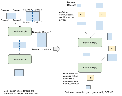
Left: A simplified feedforward layer of a Transformer model. Blue rectangles represent tensors with dashed red & blue lines overlaid representing the desired partitioning across a 2x2 mesh of devices. Right: A single partition, after GSPMD has been applied. Source: google research post.
2021 Skilful precipitation nowcasting using deep generative models of radar, Google Deepmind
Current weather predictions are done by using numerical weather predictions, by solving physical equations that descrive radar-based wind estimates. Alternative methods use machine learning to capture non-linear behaviour that is not described by the mathematical formalism of the weather-regulating equations. Two main problems arise: poor performance on rarer medium-to-heavy rain events, and weather forecast at high resolution for short-term intervals (2 hours, a.k.a. nowcasting). This paper solves demonstrates improvements in the skill of probabilistic precipitation nowcasting, by using an approach known as generative modelling, based on a deep generative model (DGM) for the probabilistic nowcasting of precipitation.
2021 Reduced, Reused and Recycled: The Life of a Dataset in Machine Learning Research, Google and Univ. California, NeurIPS 2021
Winner of the “Datasets and Benchmarks Best Paper Award” at NeurIPS 2021. Abstract: “We study how dataset usage patterns differ across machine learning subcommunities and across time from 2015-2020. We find increasing concentration on fewer and fewer datasets within task communities, significant adoption of datasets from other tasks, and concentration across the field on datasets that have been introduced by researchers situated within a small number of elite institutions.”

2021 MLP-Mixer: An all-MLP Architecture for Vision, Google, NeurIPS 2021
The paper argues that neither (CNNs) convolution CNNs or (Transformers) attention are necessary for computer vision setups. To that extent, it presents MLP-mixers, a Multi-Layer Perceptron only architecture. “MLP-Mixer contains two types of layers: one with MLPs applied independently to image patches (i.e. “mixing” the per-location features), and one with MLPs applied across patches (i.e. “mixing” spatial information).” Results are competitive with existing methods.

2021 Pay Attention to MLPs, Google, NeurIPS 2021
The paper introduces gMLP (gated MLPs) and show that they can perform as well as Transformers in language and vision applications. It claims that “self-attention is not critical for Vision Transformers, as gMLP can achieve the same accuracy”. In some BERT tasks it performed better than Transformers, and on finetuning tasks, it performed worse (but this can be overcome by making the gMLP model substantially larger).
The gMLPs have no self-attention, and instead rely on channel projections and spatial projections with static parameterization. It consists of a stack of \(L\) blocks with identical size and structure. Each block is defined as:
\[Z = σ(XU), \,\,\,\,\,\,\,\, \tilde{Z} = s(Z), \,\,\,\,\,\,\,\, Y = \tilde{Z} V\]where \(σ\) is an activation function, \(U\) and \(V\) are linear projections along the channel dimension, and \(s(·)\) is a layer which captures spatial interactions. When \(s\) is an identity mapping, the above transformation degenerates to a regular FFN, ie no cross-token communication. Here, \(s(·)\) is a spatial depthwise convolution (Section 2.1), which, unlike Transformers, does not require position embeddings because that is captured in \(s(·)\).

2021 An Image is Worth 16x16 Words: Transformers for Image Recognition at Scale, Google, ICLR 2021
Introduces Visual Transformers (ViTs), an extension of the transformer architecture to images. Works by passing as input to the transformer a sequence of linear embeddings of image patches. Paper demonstrates better results on classification tasks, compared to CNNs, ResNets and native attention mechanism (that do not scale well as pixels attend to other pixels leading to a quadratic complexity).
![]()
2021 Finetuned Language Models Are Zero-Shot Learners, Google, ICLR 2022
The paper presents a simple method for improving the zero-shot learning abilities of language models. It shows that instruction tuning – finetuning language models on a collection of tasks described via instructions – substantially improves zero-shot performance on unseen tasks. The intuition is that performing instruction tuning—finetuning of the model with datasets expressed via natural language instructions, substantially improves the zero-shot performance of the model. For each dataset, the authors manually compose ten unique templates that use natural language instructions to describe the task for that dataset.
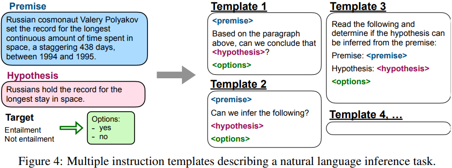
small amounts of Gaussian noise, it is sufficient to set the sampling chain transitions to conditional Gaussians too, allowing for a particularly simple neural network parameterization”.
2020 Scaling Laws for Neural Language Models, John Hopkins, OpenAI
Abstract: We study empirical scaling laws for language model performance on the cross-entropy loss. The loss scales as a power-law with model size, dataset size, and the amount of compute used for training, with some trends spanning more than seven orders of magnitude. Other architectural details such as network width or depth have minimal effects within a wide range. Simple equations govern the dependence of overfitting on model/dataset size and the dependence of training speed on model size. These relationships allow us to determine the optimal allocation of a fixed compute budget. Larger models are significantly more sample efficient, such that optimally compute-efficient training involves training very large models on a relatively modest amount of data and stopping significantly before convergence.

Keypoints:
- Model performance depends most strongly on scale, which consists of three factors: the number of model parameters N, the size of the dataset D, and the amount of compute C used for training. Performance has a power-law relationship with each of the three scale factors (Fig.1).
- Within reasonable limits, performance depends very weakly on other architectural hyperparameters such as depth vs. width.
- Performance improves predictably as long as we scale up N and D in tandem, but enters a regime of diminishing returns if either N or D is held fixed while the other increases.
- When we evaluate models on text with a different distribution than they were trained on, the results are strongly correlated to those on the training validation set with a roughly constant offset in the loss, i.e. incurs a constant penalty but improves in line with the performance of the training set.
- When working within a fixed compute budget C but without any other restrictions on the model size N or available data D, we attain optimal performance by training very large models and stopping significantly short of convergence.
- The ideal batch size for training these models is roughly a power of the loss only
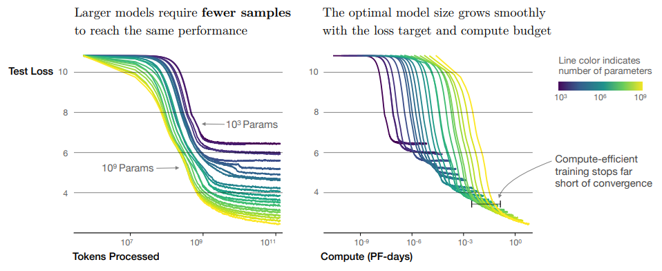
2020 Language Models are Few-Shot Learners (GPT-3), OpenAI
Up until now, substantial gains on many NLP tasks were achieved by pre-training on a large corpus of text followed by fine-tuning on a specific task. This method still requires task-specific fine-tuning datasets of thousands or tens of thousands of examples. This paper shows that scaling up language models greatly improves task-agnostic, few-shot performance, sometimes even reaching competitiveness with prior state-of-the-art finetuning approaches. This paper presents and tests GPT-3 (an autoregressive LLM with 175 billion parameters, 10x larger than previous models) in the few-shot setup.
GPT-3 architecture uses the same model and architecture as GPT-2, including the modified initialization, pre-normalization, and reversible tokenization described therein, with the exception that we use alternating dense and locally banded sparse attention patterns in the layers of the transformer, similar to the Sparse Transformer.
- Table 2.1 includes the 8 GPT-3 models built and their sizes/hyperparameters.
- Fig. 2.2 shows the total compute used during training. Based on the analysis in Scaling Laws For Neural Language Models we train much larger models on many fewer tokens than is typical.
- Fig 3.1 shows the pattern of smooth scaling of performance with compute. Performance (cross-entropy loss) follows a power-law trend with the amount of compute used for training.
Background (Fig 2.1):
- Fine-Tuning (FT) has been the most common approach in recent years, and involves updating the weights of a pre-trained model by training on a supervised dataset specific to the desired task.
- Few-Shot (FS) is the term we will use in this work to refer to the setting where the model is given a few demonstrations of the task at inference time as conditioning [RWC+19], but no weight updates are allowed.
- One-Shot (1S) is the same as few-shot except that only one demonstration is allowed, in addition to a natural language description of the task
- Zero-Shot (0S) is the same as one-shot except that no demonstrations are allowed, and the model is only given a natural language instruction describing the task.


Tasks tested and performance:
- On NLP tasks it achieves promising results in the zero-shot and one-shot settings, and in the the few-shot setting is sometimes competitive with or even occasionally surpasses state-of-the-art.
- It also displays one-shot and few-shot proficiency at tasks designed to test rapid adaption or on-the-fly reasoning, which include unscrambling words, performing arithmetic, and using novel words in a sentence after seeing them defined only once.
- Fig 3.3 to 3.12 show that GPT3’s performance grows with model size, suggesting that language models continue to absorb knowledge as their capacity increases. Results plotted for the the TriviaQA, translation, Winograd Schema Challenge, PIQA, comprehension, SuperGLUE, ANLI Round 3, arithmetic, word scrambling, and SAT tasks; on zero-, one- and few-shot training, respectively.
- Fig 3.12 shows that people’s ability to identify whether news articles are model-generated (measured by the ratio of correct assignments to non-neutral assignments) decreases as model size increases. or QuAC.
- Fig 4.2 plots the benchmark contamination analysis. Data contamination has a minimal effect on GPT-3’s performance on most datasets, but the authors identify a few datasets where it could be inflating results:
- Chaper 5 details the limitations. GPT-3 struggles with natural language inference tasks like the ANLI dataset, and some reading comprehension datasets like RACE
2020 Graph Transformers Networks, Korea University
One limitation of most GNNs is that they assume the graph structure to be fixed and homogeneous, ie similar types of nodes and edges. From the abstract: “Graph Transformer Networks (GTNs) are capable of generating new graph structures, which involve identifying useful connections between unconnected nodes on the original graph, while learning effective node representation on the new graphs in an end-to-end fashion. Graph Transformer layer, a core layer of GTNs, learns a soft selection of edge types and composite relations for generating useful multi-hop connections”.
- GTNs perform Meta-Path Generation: a meta-path defines a compositional relation over node/edge types (a sequence of relations). In the notation used in the paper, a meta-path can be written as a composed relation, e.g. \(R = t_1 \circ t_2 \circ \cdots \circ t_l\), which defines a composite relation between nodes \(v_1\) and \(v_{l+1}\).
![]()
2019 Root Mean Square Layer Normalization (RMSNorm)
RMSNorm (Root Mean Square Normalization) is a simpler and computationally efficient alternative to LayerNorm. Instead of normalizing based on the mean and variance of the input features, it only scales the input using the root mean square of the features. The benefits are (1) Efficiency: RMSNorm is computationally lighter than LayerNorm, making it ideal for large-scale models like LLaMA; and (2) Stability: its reliance on the root mean square avoids potential instabilities from mean subtraction, which can introduce noise in large dimensions. Formulated as:
\[\text{RMS}(x) = \sqrt{\frac{1}{d} \sum_{i=1}^d x_i^2}\]where \(x\) is the input vector with dimensionality \(d\), and
\[\text{RMSNorm}(x) = \frac{x}{\text{RMS}(x)} \cdot \gamma\]where \(γ\) is a learnable scaling parameter (similar to LayerNorm).
2019 Fast Transformer Decoding: One Write-Head is All You Need (Multi-Query Attention)
Efficient training in transformers model is possible due to parallelism across the length dimension. However, decoding (where such parallelization is impossible) is slow due to continuously loading large keys and values tensors into memory. Thus, this introduces a variant of the multi-head attention that improves inference (decoding), called multi-query attention. While MHA consists of multiple attention layers (heads) in parallel with different linear transformations on the queries, keys, values and outputs, MQA is identical except that the different heads share a single set of keys and values. This greatly reducing the size of these tensors and hence the memory bandwidth requirements of incremental decoding”. This leads to a much faster decoding, with minor degradation of quality from the baseline.
2019 Generating Long Sequences with Sparse Transformers, OpenAI
The paper introduces several sparse factorizations of the attention matrix that reduce the quadratic complexity on memory and runtime Transformers to \(O(n \sqrt{n})\). It also allows for larger sequences. These work by separating the full attention computation into several faster attention operations which, when combined, can approximate the dense attention operation. The authors claim that sparsity in attention is a natural pattern and show (by visual inspection) various examples where most layers had sparse attention patterns across most data points, suggesting that adding sparsity to the attention would not signficantly affecting performance. In other layers, however, they noticed global patterns and data-dependent sparsity, whose performance could be affected by sparsity in the attention matrix.
Factorized self-attention proposes \(p\) separate attention heads, where each head handles a subset of the indices. The hard problem here is to find efficient choices for the subset \(A\). Section 4.3 details 2D factorization methods via strided attention, or fixed patterns (figure below).
![]()
2019 ALBERT: A Lite BERT for Self-supervised Learning of Language Representations, Google and Toyota
ALBERT (“A Lite BERT”) lowers memory consumption and increase the training speed of BERT. It allows for better scaling, establishes new record performance in several benchmarks, and with fewer parameters than BERT. An ALBERT configuration similar to BERT-large has 18x fewer parameters and can be trained about 1.7x faster. The tecnniques introduced are:
- Factorized embedding parameterization, for parameter reduction. “Instead of projecting the one-hot vectors directly into the hidden space of size \(H\), we first project them into a lower dimensional embedding space of size \(E\), and then project it to the hidden space. By using this decomposition, we reduce the embedding parameters from \(O(V × H)\) to \(O(V × E + E × H)\)”. This separation of the size of the hidden layers from the size of vocabulary embedding, makes it easier to grow the hidden size without significantly increasing the parameter size of the vocabulary embeddings.
- Cross-layer parameter sharing, for parameter reduction. The authors mention that the parameter reduction also acts as regularisation/generalisation (reduces overfitting as the model learns a representation that generalizes well for all tasks). It does not improve the performance of the model though: “This approach slightly diminishes the accuracy, but the more compact size is well worth the tradeoff”. This technique prevents the parameter from growing with the depth of the network. As a practical example, take a BERT model with 12 layers ie 12 Transformer encoder blocks: instead of learning unique parameters for each layer, ALBERT learns parameters of the first layer reuse the block in the remaining 11 layers.
- Self-supervised loss for sentence-order prediction (SOP), for performance improvement. Instead of BERT’s additional loss called next-sentence prediction (NSP, a binary classification loss for predicting whether two segments appear consecutively in the original text), the authors propose SOP, focused on inter-sentence coherence which is designed to address the ineffectiveness of the NSP in BERT. The SOP loss uses as positive examples the same technique as BERT (two consecutive segments from the same document), and as negative examples the same two consecutive segments but with their order swapped. This forces the model to learn finer-grained distinctions about discourse-level coherence properties.
2018 Averaging Weights Leads to Wider Optima and Better Generalization (Stochastic Weight Averaging), Cornel & Samsumg AI
The authors present SWA, a “simple averaging of multiple points along the trajectory of SGD, with a cyclical or constant learning rate, that leads to better generalization than conventional training” and provides “much flatter solutions than SGD”. The rationale is: (1) SGD with constant or cyclical LR traverse regions of weight space that correspond to high-performing networks, never reaching their central points. (2) Fast Gradient Ensembles (FGE) for \(k\) models required \(l\) times more computation. SWA is an approximation of FGE with the efficiency of a single model, with a better solution that SGD. The algorithm is the following: Starting from \(\hat{w}\) we continue training, using a cyclical or constant learning rate schedule:
-
When using a cyclical learning rate we capture the models \(w_i\) that correspond to the minimum values of the learning rate, i.e. the values at then end of each cycle (at the lowest learning rate value);
-
For high constant learning rates we capture models at each epoch.
Next, we average the weights of all the captured networks \(w_i\) to get our final model \(w_{SWA}\). For cyclical learning rate schedule, the SWA algorithm is related to FGE, except that instead of averaging the predictions of the models, we average their weights, and we use a different type of learning rate cycle.
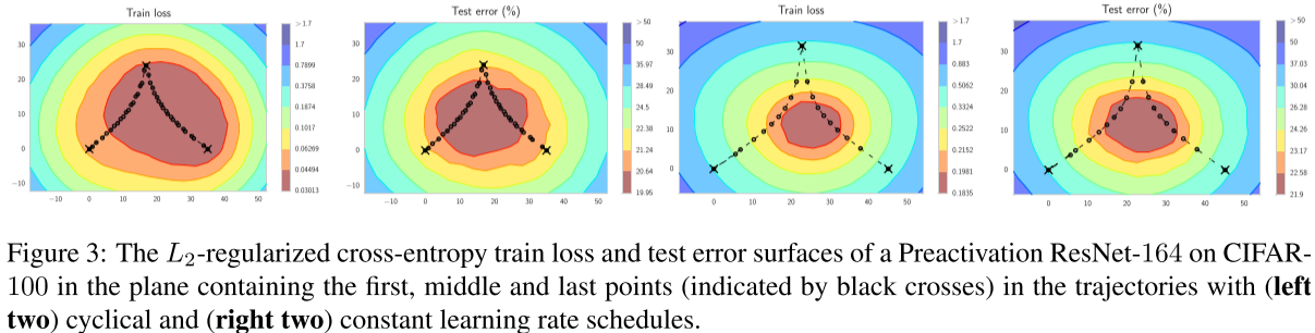
2017 Neural Discrete Representation Learning (RQVAE), Google
The Vector Quantised Variational AutoEncoder (VQ-VAE) aims at learning discrete (not continuous) latent space representations without supervision. It differs from VAEs in two key ways: the encoder network outputs discrete, rather than continuous, codes; and the prior is learnt rather than static. “During forward computation the nearest embedding \(z_q(x)\) (equation 2) is passed to the decoder, and during the backwards pass the gradient \(∇_z\)L is passed unaltered to the encoder. Since the output representation of the encoder and the input to the decoder share the same \(D\) dimensional space, the gradients contain useful information for how the encoder has to change its output to lower the reconstruction loss.” Equation 3 specifies the overall loss function, which has some tricks to allow the model to learn from the discrete mapping of mapping from \(z_e(x)\) to \(z_q(x)\).
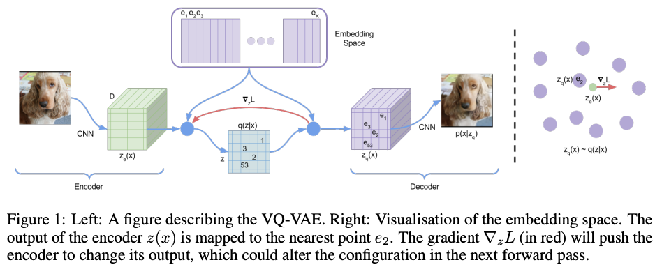
2017 Mixed Precision Training, Baidu and NVIDIA
A method for training using half-precision floating point numbers, without losing model accuracy or having to modify hyperparameters. Due to the reduced range of 16- vs 32-bit representation, three techniques are proposed to prevent the loss of critical information (or numerical overflows):
- Maintaining a single-precision copy of weights that accumulates the gradients after each optimizer step. This copy must then be rounded to half-precision for the forward- and back-propagation.
- performing loss-scaling to preserve gradient values with small magnitudes. To implement scaling, scale the loss value computed in the forward pass by shifting the gradient values into FP16-representable range, prior to back-propagation. Weight gradients must be unscaled before weight update to maintain the update magnitudes as in FP32 training.
- Using half-precision arithmetic that accumulates into single-precision outputs, which are converted to half precision before storing to memory. Different arithmetics (vector dot-products, reductions, and point-wise operations) require different treatment.
2018 Group Normalization, Facebook AI Research
This paper presents Group normalization. GN surpasses Batch Normalization particularly on small batch sizes, due to error increasing rapidly when the batch size becomes smaller. Layer Normalization and Instance Normalization also avoid normalizing along the batch dimension. These methods are effective for training sequential models (RNN/LSTM) or generative models (GANs), but both have limited success in visual recognition, for which GN presented better results.
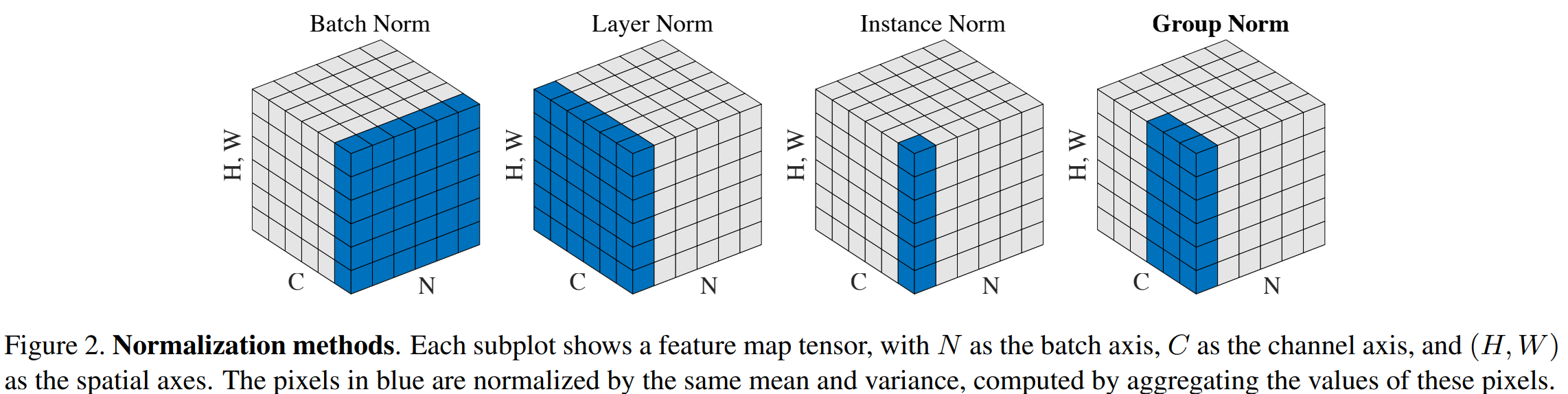
2016 Semi-Supervised Classification with Graph Convolutional Networks
Introduces GraphConvNets (GCNs), a variant of the Convolutional Neural Networks that operate on graphs. Similarly to CNNs, GCNs learn the features by inspecting neighboring nodes. The main difference is that CNNs are meant to operate on regular Euclidean structures (e.g. images), while GNNs are a generalized applicable to an arbitrary structure or order.

2016 Neural Architecture Search with Reinforcement Learning, Google, ICLR 2017
Neural Architecture Search (NAS) is a subfield of machine learning that focuses on automating the design of neural network architectures. Instead of manually designing the structure of a neural network (e.g., number of layers, number of neurons per layer, type of activation functions), NAS uses algorithms to search for optimal architectures within a defined search space.
The authors propose “a recurrent network to generate the model descriptions of neural networks and train this RNN with reinforcement learning to maximize the expected accuracy of the generated architectures on a validation set.” Basically, a DNN that defines the structure of another DNN using RL. The structure and connectivity of the model being designed (the child network) is represented as a variable-length string. This string is generated by the controller network - a recurrent neural network - that uses the child network’s accuracy on the validation set as a reward signal.
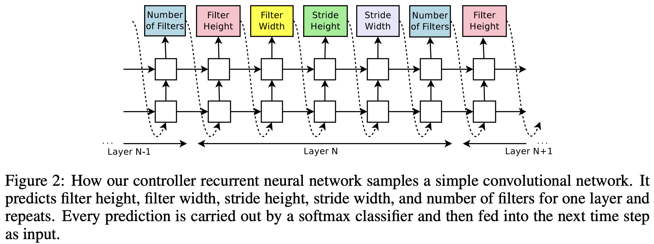
2015 Batch Normalization: Accelerating Deep Network Training by Reducing Internal Covariate Shift
Batch Normalization (BatchNorm) is a technique used in deep learning to improve the training process of neural networks by normalizing the inputs to each layer within a mini-batch. It “reduces the internal covariate shift”. Covariate shift means the distribution of the features is different in different parts of the training/test data, breaking the i.i.d assumption used across most of ML. This happens because, as the network learns and the weights are updated, the distribution of outputs of a specific layer in the network changes. This forces the higher layers to adapt to that drift, which slows down learning. BN helps by making the data flowing between intermediate layers of the network look like whitened data, this means you can use a higher learning rate. In the results, Batch Normalization achieves the same accuracy with 14 times fewer training steps, and beats the original model by a significant margin.
2015 Siamese neural networks for one-shot image recognition, CS Toronto, ICML 2015
The paper describes siamese neural networks (see below for details) for efficient one-shot learning. General strategy. 1) Train a model to discriminate between a collection of same/different pairs; 2) Generalize to evaluate new categories based on learned feature mappings for verification. The architecture of each siamese network is a convolutional neural network, with a flattening and a feed-forward network in the head. The loss functions is a binary cross-entropy with a regularizer.
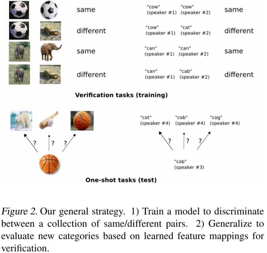 \(\, \, \,\)
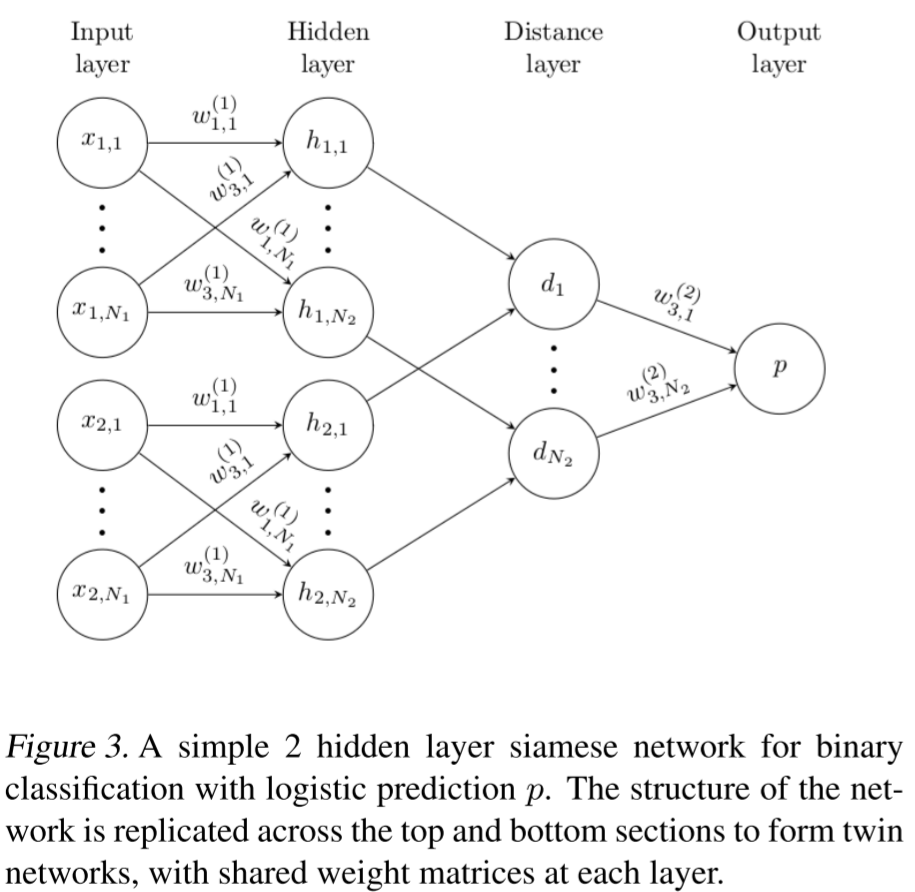
2015 Neural Machine Translation by Jointly Learning to Align and Translate (and Attention Mechanism), D. Bahdanau, K. Cho, Y. Bengio
An improvement of the sequence-to-sequence translation work in Sequence to Sequence Learning with Neural Networks (Google, arXiv)). Introduces the concept of attention and improves translation performance by utilising the latent space of every encoder iteration (not just the last) on the decoding steps, in order to increase the model capatiblities


2014 Deeply-supervised Nets, USCD and Microsoft
A deeply supervised model in machine learning refers to a model architecture where intermediate layers are explicitly supervised during training, in addition to the supervision applied to the final output layer. This technique encourages better learning throughout the model by enforcing that earlier layers learn features useful for solving the task directly, rather than solely relying on gradients propagated from the final layer.
Deep supervision was introduced to address challenges such as vanishing gradients, poor feature learning in intermediate layers, and inefficiency in deep networks. It is particularly common in tasks like image segmentation, object detection, and biomedical image analysis.
The objective of the intermediate layers is called the “companion objective”, which is used as an additional constraint (or a new regularization) to the learning process. Example: Adding an parameter “\(γ\) as a threshold (a hyper parameter) … with a hinge loss: once the overall value of the hidden layer reaches or is below \(γ\), it vanishes and no longer plays role in the learning process. … The empirical result suggests the following main properties of the companion objective: (1) it acts as a kind of feature regularization (although an unusual one), which leads to significant reduction to the testing error but not necessarily to the train error; (2) it results in faster convergence, especially in presence of small training data”
2014 Dropout: a simple way to prevent neural networks from overfitting, Univ. Toronto, Journal of ML Research 2014
A method that drops neurons (in different layers) with a given probability \(p\) during train time. For each training minibatch, a new network is sampled. Dropout can be improved by adding max-norm regularization, decaying learning rate and high momentum. At test time, all neurons are used, with outgoing weights multiplied by \(p\). Dropout helps reducing overfitting, as the network learns to never rely on any given activations, so it learns “redundant” ways of solving the task with multiple neurons. It also leads to sparse activations, similar to a regularization (L2). Dropping 20% of input units and 50% of hidden units was often found to be optimal in the original publication. It’s computationally less expensive than regular model averaging of multiple trained DNNs. However, it takes 2-3 times longer to train than single fully-connected DNNs because requires way more epochs, as parameter updates are very noisy. Because a fully connected layer occupies most of the parameters, it is prone to overfitting. Therefore, dropout increases model generalization.
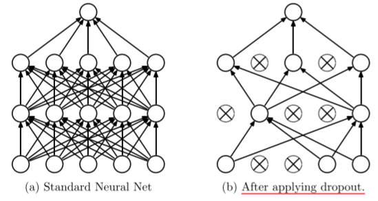
2011 Popular Ensemble Methods: An Empirical Study, 2011
A summary of results and conclusions on ensemble methods (bagging, boosting) on DNNs and decision trees. Bagging ensemble generally produces a classifier that is more accurate than a standard classifier. About Boosting: for a few data sets Boosting produced dramatic reductions in error (even compared to Bagging), but for other data sets it actually increases in error over a single classifier (particularly with neural networks). Alternatively, an ensemble of similar DNNs initialized with different random seeds is surprisingly effective, often producing results as good as Bagging. An ideal ensemble consists of highly correct classifiers that disagree as much as possible.
Bagging trains the several different models with different datapoints randomly sampled (with replacement, ie same samples can be redrawn) from the same dataset. Bagging is effective on “unstable” learning algorithms (such as DNNs) where small changes in the training set result in large changes in predictions.
Boosting produces a series of classifiers. The training set used for each member of the series is chosen based on the performance of the earlier classifier(s) in the series. Examples that are incorrectly predicted by previous classifiers in the series are chosen more often than those correctly predicted. Thus Boosting attempts to produce new classifiers that are better able to predict examples for which the current ensemble’s performance is poor. Ada-Boosting can use the approach of (1) selecting a set of examples based on the probabilities of the examples, or (2) simply using all of the examples and weight the error of each example by the probability for that example (i.e., examples with higher probabilities have more effect on the error) – easier as these probabilities are incorporated in the dataset.

2011 Cyclical Learning Rates for Training Neural Networks, US Naval Research Lab, 2017
The author claims that cyclic learning rates improve time to convergence and increases accuracy of most models. It suggests triangular scheduler as a efficient method with similar results to other non-triangular cyclic schedulers. The paper also provides a method to find a good initial learning rate by doing several training short sessions (8 iterations) with different learning rates and picking the best initial learning rate from the analysis. Finally, provides “rule of thumb” parameters for min and max learning rates in the triangular scheduler proposed.
2006 Dimensionality Reduction by Learning an Invariant Mapping (contrastive loss), New York Uni, CVPR 2006
The paper presents Dimensionality Reduction by Learning an Invariant Mapping (DrLIM). The problem is to find a function that maps high dimensional input patterns to lower dimensional outputs, given neighborhood relationships between samples in input space. It presents the Contrastive Loss Function. The contrastive loss trains 2 siamese networks, and encourages the model to learn a representation space where similar samples are close together, and dissimilar samples are far apart. A Siamese Network is a type of neural network architecture designed to compare two inputs by learning their similarity or relationship. It consists of two identical subnetworks (hence the name “Siamese”) that share the same architecture and weights. Each subnetwork processes one of the two inputs independently, and the outputs are then combined to compute a similarity score or distance metric. The input to system is a pair of images (one to each of the siamese networks) and the dissimilarty label (0 for dissimilar images or 1 for similar images). The images are passed through the functions, yielding two outputs \(G(X_1)\) and \(G(X_2)\). The cost module then computes the euclidian distance between both outputs as \(D_W(G_W(X_1), G_W(X_2))\). The objective is formulated in terms of the similarity label \(y\) (1 for similar, 0 for dissimilar) and the euclidian distance \(D\) between the two images as:
\[L = \frac{1}{2} ⋅y⋅D^2 + \frac{1}{2} ⋅(1−y)⋅max(0,m−D)^2\]where \(m\) is a margin hyperparameter that sets the minimum distance for dissimilar pairs. The architecture is a siamese architecture, two copies of the same network which share the same set of parameters, and a cost module. The total gradient is the sum of the contributions from the two instances.