Variable Timestep Simulation of the Electrical Activity of Neurons
In the previous post, I detailed the mathematical background underlying neurons activity. Then I detailed the simulation of the electrical activity of simple neuron models, and mentioned that an interleaved voltage-current resolution of linear unrelated state ODEs allows for the resolution of the problem as a system of linear equations. However, such resolution is only possible for those simple models. Neuron models with non-linear state variable OPDEs and correlation between states require a fully-implicit resolution, and is possible with Backward Euler with Newton iterations. This is a common use case, and underlies the resolution of extra-cellular mechanisms, capacitors between nodes, and other mechanisms that connect neurons’ evolution over time.
A fully-implicit method that is commonly utilised to resolve this problem is the Backward (Implicit) Euler, where:
\[y_{n+1} - y_n = h f (t_{n+1}, y_{n+1})\]where \(h\) is the timestep, \(y\) is the array of states and \(f\) is the Right-Hand side function of the ODE. Can we do better? In this post we present a fully-implicit method based on variable-order variable timestepping.
CVODE for fully-implicit adaptive-order adaptive-step interpolation
The main principle supporting the adaptive time stepping is its particular efficiency due to a large step size upon large and low-varying states e.g. interspiking intervals. NEURON’s adaptive algorithm, CVODE uses separate variable-step integrators for individual neurons in the network. CVODE is used by NEURON as an interface to a collection of methods built on top of existing CVODE and IDA (Integrator for Differential-Algebraic problems) integrators of the SUNDIALS package, a SUite of Nonlinear and DIfferential/ALgebraic Equation Solvers. NEURON employs the Backward Differentiation Formula. The backward differentiation formula is a family of implicit multi-step methods for the numerical integration of (stiff) ordinary differential equations. For a given function and time, the BDF approximates its derivative using information from previously computed times, thus increasing the accuracy of the approximation. BDF methods are implicit thus require the computing the solution of nonlinear equations at every step. The BDF multistep method is suitable for stiff problems that define neuronal activity. The main idea behind a stiff equation is that the equation includes terms that may lead to rapid variation of the solution, therefore causing certain numerical methods for solving the equation numerically unstable, unless the step size is taken to be extremely small. CVODES is a solver for the Initial Value Problem — the IVP is an ODE together with an initial condition of the unknown function at a given point in the domain of the solution — that can be written abstractly as:
\[\dot{y} = f(t,y) \text{, } y(t_0) = y_0 \text{ where } y \in \mathbb{R}^N\]where \(\dot{y}\) denotes \(\frac{dy}{dt}\). The solution \(y\) is differentiated using past (backward) values, ie \(\dot{y}_n\) is the linear combination of \(y_n\), \(y_{n-1}\), \(y_{n-2}, ...\). \(y\) is the array of all state variables, in our case the \(dV_n/dt\) equation of all compartments, and \(dx_i/dt\) where \(x_i\) is a given state variable of an ion \(i\). The variable-step BDF with \(q\)-order can be written as:
\[y_n = \sum_i^{q} \alpha_{n,i} y_{n-i} + h_n \beta _{n,0} \dot{y}_n\]where \(y_n\) are computed approximations to \(y (t_n)\), \(h_n = t_n - t_{n-1}\) is the step size, \(q\) denotes the order (number of previous steps used on BDF), and \(\alpha\) and \(\beta\) are the unique coefficients of BDF dependent on the method order. The resolution can be unfolded as:
- BDF-1: \(y_{n+1} - y_n = h f (t_{n+1}, y_{n+1})\), i.e. the Backward Euler;
- BDF-2: \(3y_{n+2} - 4y_{n+1} + y_n = 2 h f (t_{n+2}, y_{n+2})\);
- BDF-3: \(11y_{n+3} - 8y_{n+2} + 9y_{n+1} - 2y_n = 6 h f (t_{n+3}, y_{n+3})\);
- BDF-4: \(25y_{n+4} - 48y_{n+3} + 36y_{n+2} - 13y_{n+1} + 3y_n = 12 h f (t_{n+4}, y_{n+4})\);
- BDF-5: \(137y_{n+5} - 300y_{n+4} + 300y_{n+3} - 200y_{n+2} + 75y_{n+1} - 12y_n = 60 h f (t_{n+5}, y_{n+5})\);
- BDF-6: \(147y_{n+6} - 360y_{n+5} + 450y_{n+4} - 400y_{n+3} + 225y_{n+2} - 72y_{n+1} + 10y_n = 60 h f(t_{n+6}, y_{n+6})\);
BDF with order \(q > 7\) is not zero-stable therefore is unable to be used. If a perturbation \(\epsilon\) happens on an initial value, then final result between perturbed and unperturbed results must be no bigger than \(k \epsilon\), for any \(k \in \mathbb{R}\)} therefore cannot be used. CVODE allows for a maximum order or 5.
If we denote the Newton iterates by \(y_{n,m}\), the functional iteration of the BDF is given by:
\[y_{n,m+1} = h_n \beta _{n,0} f ( t_n, y_{n,m} ) + a_n \label{eq_newton_method_derivation}\]As with any implicit method, at every step we must (approximately) solve the nonlinear system:
\[G(y_n) \equiv y_n - h_n \beta_{n,0} f(t_n, y_n) - a_n = 0 \text{ , where } a_n \equiv \sum_{i>0} ( \alpha_{n,i} y_{n-1} + h_n \beta_{n,i} \dot{y}_{n-i} ) \label{eq_variable_time_step_bdf}\]To resolve this, CVODE applies Newton iterations. The Newton’s method allows to finding successively better approximations to the roots or zeroes of a function, and is implemented (for one variable) as \(x_{n+1} = x_n - f(x_n) / f'(x_n)\) until a sufficiently accurate value is reached. In practice, it requires finding the solution of the linear systems:
\[M [y_{n(m+1)} - y_{n(m)}] = - G(y_{n(m)})\]where
\[M \approx I - \gamma J \text{ , } J = \partial f / \partial y \text{ , and } \gamma = h_n \beta_{n,0}\]For the Newton corrections, CVODE provides the following options: (a) direct dense solver, (b) direct banded solver, (c) a diagonal approximate Jacobian solver, or the SPGMR (Scaled Preconditioned GMRES) method. A preconditioner matrix is a transformation that conditions a given problem into a form that is more suitable for numerical solving methods. NEURON applies the SPGMR method, that requires a matrix \(M\) (or preconditioner matrix \(P\) for the SPGMR case) to be an Inexact Newton iteration, in which \(M\) is applied in a matrix-free manner, where the matrix-vector products \(Jv\) are obtained by either difference quotients or an user-supplied routine. In NEURON, \(J y\) is user-provided by the SOLVE block in the mechanisms. In practice, the SPGMR transforms the nonlinear problem into a linear one, by introducing a multiplication by the Jacobian (In vector calculus, the Jacobian matrix is the matrix of all first-order partial derivatives of a vector-valued function), and it involves computing the solution of the equation:
\[\begin{align*} y_{n(m+1)} = & y_{n(m)} - J^{-1} G(y_{n(m)}) \\ \equiv & y_{n(m+1)} - y_{n(m)} = - J^{-1} G(y_{n(m)}) \\ \equiv & P [y_{n(m+1)} - y_{n(m)}] = - P J^{-1} G(y_{n(m)}) \\ \equiv & P [y_{n(m+1)} - y_{n(m)}] = - G(y_{n(m)}) \\ \end{align*}\]where
\[P \approx I - \gamma J \text{ , } J = \partial f / \partial y \text{ , and } \gamma = h_n \beta_{n,0}\]The previous equation requires a division by the Jacobian \(J\), i.e. a multiplication by its inverse. Due to the expensive computation of the inverse of the Jacobian, CVODE allows for a trade-off of accuracy and solution time of any equation, by requiring one to only supply a solver for \(P y = b\) instead. For the linear case, although NEURON supports a resolution with the Hines solver (default) or the (a) or (c) methods mentioned previously, there has been little exploration of the non-Hines approaches.
Error Handling
One main difference between fixed and variable time stepping, is that from the user’s perspective, one does not specify the time step but the relative local (rtol) and absolute errors (atol) instead. The solver then adjusts \(\Delta t\) based on the two values. The local error is based on the extrapolation process within a time step. CVODE uses a weighted root-mean-square norm for all error-like quantities, denoted as:
\[|| v || = \sqrt{ \frac{1}{N} \sum_{i=1}^N (v_i / W_i)^2}\]where \(v_i\) represent the deviations and the weights \(W_i\) are based on the current solution (with components \(y^i\)), with user-specified absolute tolerances \(atol_i\) and relative tolerance \(rtol\) as:
\[W_i = rtol \cdot | y^i | + atol_i\]If \(y_n\) is the exact solution of equation \ref{eq_newton_method_derivation}, we want to ensure that the iteration error is small enough such that \(y_{n,m} - y_{n,m-1} < 0.1 \epsilon\) (where \(0.1\) is user-changeable). For this, we also estimate the linear convergence rate constant \(R\), initialized at \(1\) and reset to \(1\) when \(M\) or \(P\) is updated. After computing a correction \(\delta_m = y_{n(m)} - y_{n(m-1)}\), we update \(R\) if \(m > 1\) as:
\[R \leftarrow \text{max} \left\{ 0.3 R, \frac{|| \delta_m ||}{||\delta_{m-1} ||} \right\}\]We use it to estimate
\[||y_n - y_{n(m)}|| \approx || y_{n(m+1)} - y_{n(m)}|| \approx R || y_{n(m)} - y_{n(m-1)}|| = R || \delta_m ||\]Thus, the convergence test is
\[R || \delta_m || < 0.1 \epsilon\]Local and Global Time Stepping
NEURON’s default error setting for CVODE is \(10 \mu M\) for membrane potential and \(0.1 nM\) for internal free calcium concentration, allowing a HH-based action potential to have an accuracy equivalent of fixed time step with \(\Delta t = 25 \mu s\). The default maximum order for BDF is \(5\), although it is recommended to let CVODE decide the best order.
Large networks of cells can not be integrated by a global adaptive time stepping, as a high frequency of events such as gating channels or synapses causes a discontinuity in a parameter or state variable, therefore requiring the reinitialization of computation and forcing the integrator to start again with a new initial condition problem.NEURON’s workaround allows for a local variable time stepping scheme called lvardt (Lytton et al., Independent Variable Time-Step Integration of Individual Neurons for Network Simulations, MIT Press) that creates individual CVODE integrators per cell and aims at short time step integration for active neurons and long time step integration for inactive neurons, while maintaining consistent the integration accuracy. All cells are on a ordered queue with its position given by event delivery time or actual time of simulation. Because the system’s integrator moves forward in time by multiple, independent integrators, the overall computation is reduced when compared to the global counterpart. Nevertheless, the main issue is the coordination of time advancement of each cell, i.e. all the state variables for a given cell should be correctly available to any incoming event. To solve that issue, every cell holds the information for all states between its current time instant and the previous time steps. This allows for backward interpolation when required. The integration coordinator also ensures that the interpolation intervals of the connected cells overlap, so that no event between two cells is missed. The critical point of this approach is that the time step is tentative, and an event received by the cell in the interim may reinitialize the cell to a time prior to the tentatively calculated threshold time.
In the following picture, we illustrate A time line (from A to D) of six cells running the lvardt algorithm. The intervals of possible interpolation are displayed as a black rectangle. The system’s earliest event time is shown by the vertical line traversing all neurons. Triggers of discrete events on a particular neuron are displayed as a short thick vertical bar. (A) the smallest \(t_b\) advances by the length of the hashed rectangle; (B) Cell 5 has the smallest \(t_bb\) and integrates forward; (C) The next earliest event on the system is at neuron 3. This event trigger creates three new events to be delivered to cells 3,4,5; (D) The new early event forces cell 3 back-interpolates, the event is handled, and cell 3 reinitializes. Cell 3 will be the next cell to integrate forward:
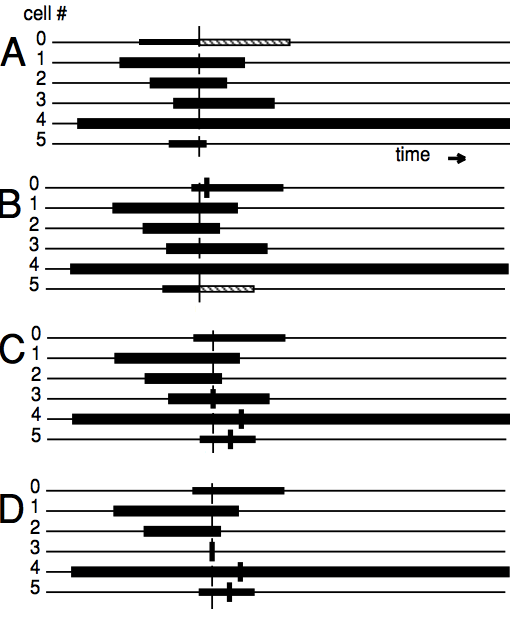
source: [The NEURON book][neuron-book]
Single Neuron Performance
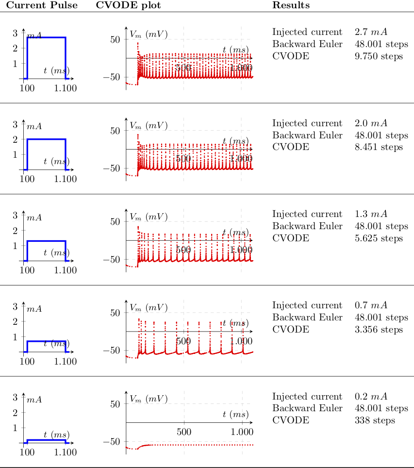
One can notice the difference in performance of the Backward Euler and Variable Timestep interpolators during a stiff trajectory of an Action Potential in the following picture.

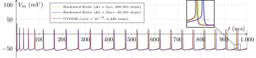
Note the difference in interpolation instants, placed at a equidistant interval on the Backward Euler use case, and adapting to solution gradient on the variable step counterpart. A current injection at the soma forces the neuron to spike at a rate that increases with the injected current. A simple consists in measuring the number of interpolations betweeen both methods, by trying to enforce different levels of stiffness and measure the number of steps:
The slow dynamics of the fixed step method — that end up accounting for the events at discrete intervals instead of event delivery times of its variable step counterpart — lead to a propagation of voltage trajectory (you can assume Euler with \(\Delta t=1 \mu s\) and \(CVODE with atol=10^{-4}\) as reference solutions):
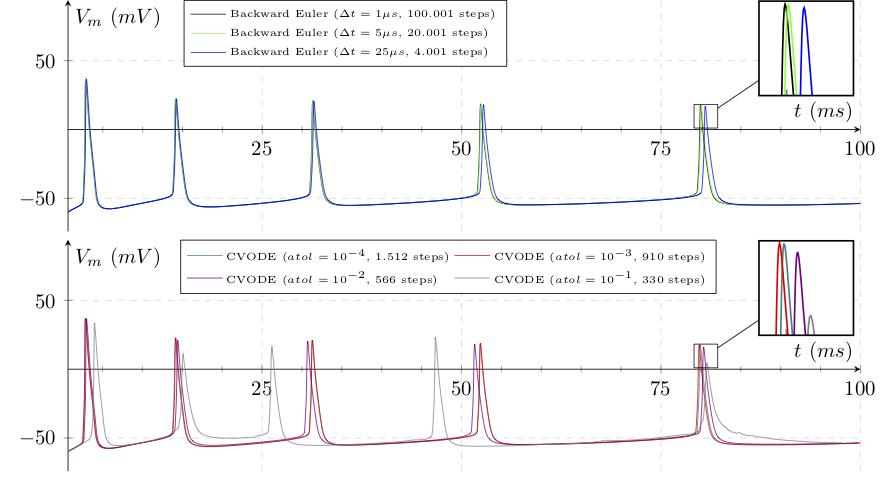
After a second of simulation, the spike time phase-shifting is substantial, demonstrating the gain in using variable step methods for this use case.
To study wether these advantages are feasible, we measure the simulation runtime of both methods. Our first test measures the impact of the stiffness in terms of simulation steps and time to solution on an intel i5 2.6Ghz. The different current values are injected as proportional to the action potential threshold current, i.e. the minimum current that is required to be continuously injected for the neuron to spike.
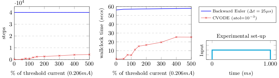
Results look promising, even at an extremelly high current value we have a significant speed-up. A second test enforces discontinuities and reset of the IVP problems by artificially injecting current pulses of \(1 \mu s\) at given frequencies.

In this scenario, we see a high dependency on the number of discontinuities, and some yet minor dependency on the discontinuity value (i.e. amount of current injected). The holy grail is then in: How does this apply to networks of neurons?
Simulation of a network of homegeneous neurons
The performance of lvardt’s integration model was tested (Lytton et al. 2015) on a connected homogeneous network of 100 inhibitory neurons on a single compute node. Due to their inhibitory features, the circuit presents rapid synchronization through mutual inhibition, where variable time steps integrators are likely to encounter problems. A fixed time step of \(0.0025 ms\) yielded closely comparable results to those of lvardt with absolute error tolerance (atol) of \(10^{-3}\) or \(10^{-5}\). The event deliveries and the associated interpolations took about \(12\%\) of total execution time. When using lvardt’s global time stepping, the author claims the large amount of events lead to an increase of execution time in the order of 60-fold. Another experiment featured a Thalamocortical simulation, featuring four cell types (cortical pyramidal neurons and interneurons, thalamocortical cells, and thalamic reticular neurons). The two thalamic cell types produced bursts with prolonged interburst intervals, therefore very suitable for the use of the lvardt algorithm. A simulation of \(150 ms\) of simulation time, aiming at high-precision with an error tolerance (atol) of \(10^{-6}\) for lvardt and \(\Delta t = 10^{-4} ms\) for the fixed time step, yielded an execution time of 6 minute 13 seconds and 10 hour 20 minute, respectively, a 100-fold speed-up. For a standard-precision run, with an atol of \(10^{-3}\) and \(\Delta t = 10^{-2}\), the simulations took 2 minutes for lvardt and 5 minutes 53 seconds for fixed time step, a 3-fold speed-up.
In the following picture we present the afforementioned results for the comparison of fixed and variable time step methods for the mutual-inhibition model. Execution time grows linearly with simulation time for the fixed-step integration (dashed lines). Variable-step methods have a reduction in CPU load at the onset of synchrony. The rationale behind the non-linearity of adaptive time stepping, is that lvardt produces time steps that jump around during the initial presynchrony phase of the simulation (fast uprising phase), and then slowly stabilizes to an alternation between large steps in the long intervals separating the population spikes and extremely short time steps during the population spike itself:
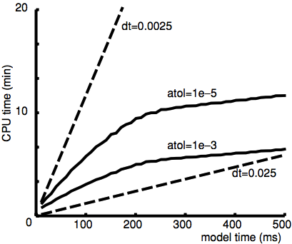
source: Lytton et al. 2015
Simulation of a network of heterogeneous neurons
Although network of similarly-behaving neurons guive us an estimation of achievable speed-up when using fixed and variable time step interpolations, it is a rough estimation. In practice, the brain activity differs widely across space and time.
To measure the efficiency across the different spiking dynamics across neurons, we reproduced a previously-published digital reconstruction of a laboratory experiment from the Blue Brain Project on the Cell Magazine. We simulated 7.5 seconds of electrical activity, performing a fixed-step simulation of the spontaneous activity of 219.247 neurons during tonic depolarization. For the biology enthusiasts: the network exhibits spontaneous slow oscillatory population bursts, initiated in Layer 5, spreading down to L6, and then up to L4 and L2/3 with secondary bursts spreading back to L6. For further details, refer to section \textit{Simulating Spontaneous Activity} in \cite{markram2015reconstruction}.
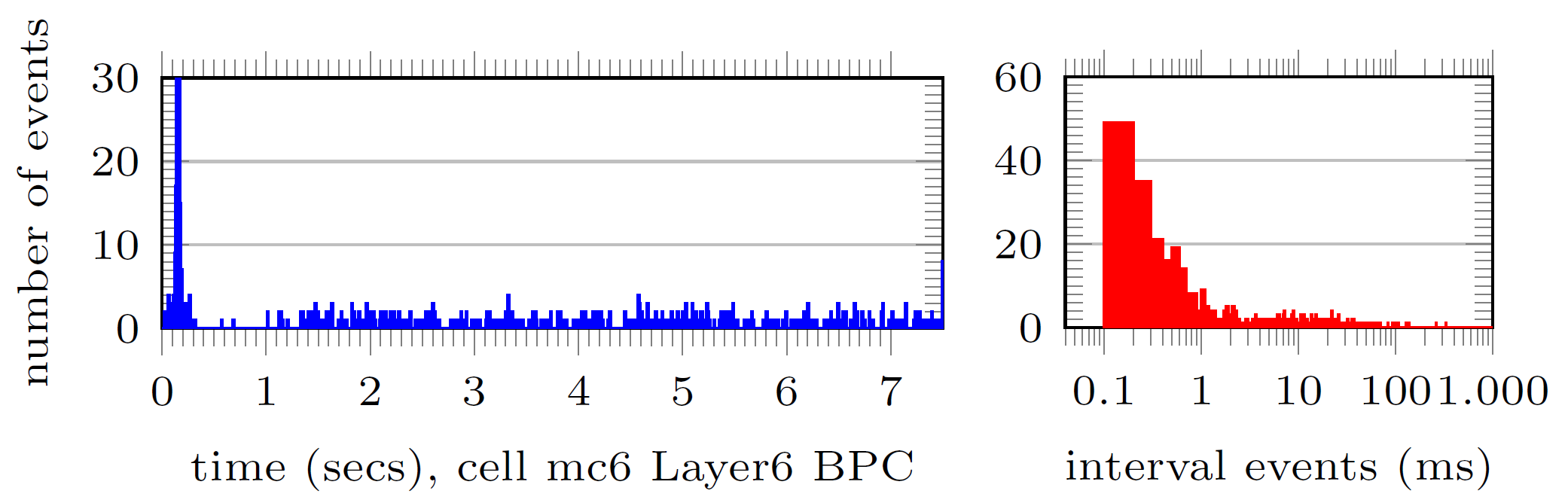
We take two sample neurons from the top 1% busiest neurons (in terms of incoming spikes i.e. discontinuities) and visually analyse the number of spikes arriving per time interval (left, each time bin account for 0.1ms) and the distribution of time intervals between spikes arrival (right):


The number of spikes received in that top 1% was between 3040 and 6146 events. We redo the same analysis for two sample neurons collected from the mean 1% of neurons in terms of spiking arrivals:

With 541 to 558 spiking events. And the bottom 1%:
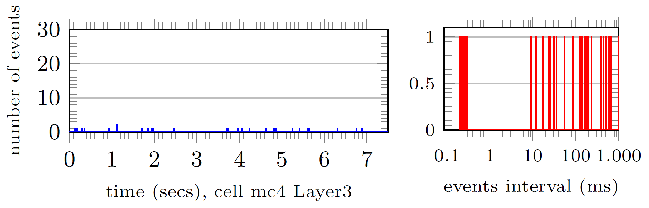
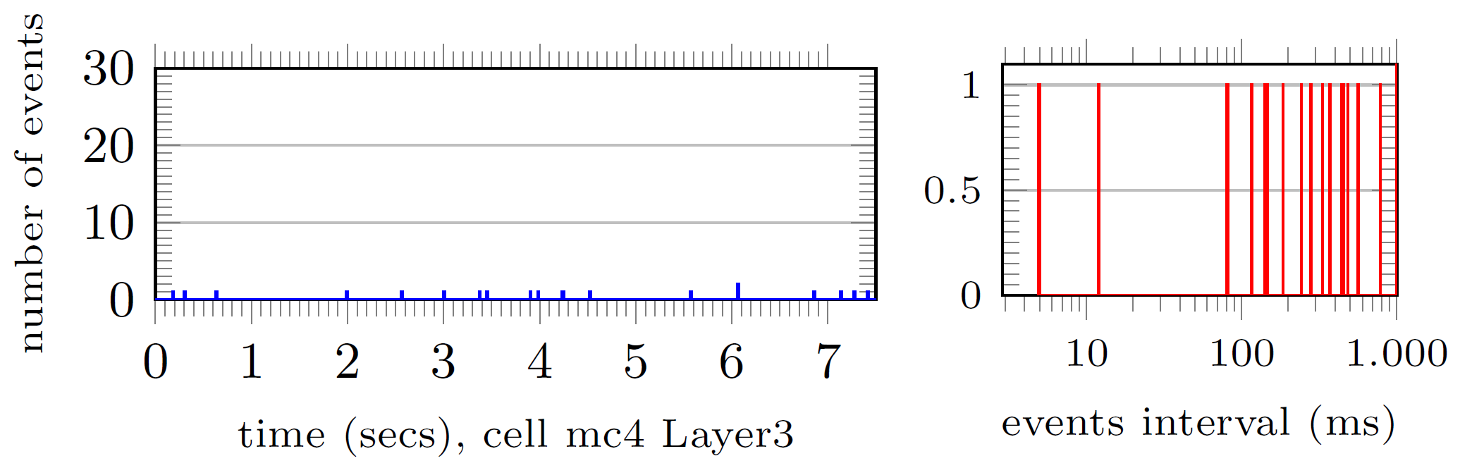
with less than 100 events.
The total events received across all neurons in the network was of approximately 155 Million, i.e. mean per neuron of 707 current spikes received. In practice, this means that most brain regions (or pattern activities) fall within the interval of acceleration that we described in the previous section.
Is the theoretical speed-up guaranteed to hold in practice? As Einstein once said “In theory, there’s no difference between theory and practice, but in practice, there is”. And that’s exactly right in our case, where two main issues arise.
1. Distributed CVODE executions
Simulations of such scale require parallel/distributed computing due to the memory/computation requirements.
However, for parallel computing environments, the synchronization of cells spread across different computing nodes presents a bottleneck, due to the required step synchronization between neurons. In practice, neurons held on different compute nodes have to able to communicate their time instant, so that when they spike, the synaptic current is delivered to a second neuron that has not advanced ahead of the delivery time (or the spike would be missed.
To tackle this issues, simulation is split in equidistant time intervals equal to the shortest delay of any global event — typically the minimal synaptic delay across all synapses, or (when applicable) the update frequency for extra-cellular mechanisms or gap junctions. On every time interval, all the nodes on the network perform a collective communication call and share the events (spikes) to be sent on the next time frame. This approach has demonstrated previously (Lytton et al. 2015) to provide a good speed-up. We can then guarantee:
- Asychronous computation: every core in every compute node computes their dataset (neurons) independently, and advances the neurons until the time limit of the next synchronization interval;
- Asynchronous communication: synaptic activity can be transmitted immediatly after they occur or together with the synchronization information in an all-to-all communication;
- Synchronous communication: neurons interpolation and spikes communication for a stepping time-window must be completed until computation and communication for the next window starts.
However, going to the extreme of the possible optimisation, we observe that this colective synchronization of neurons has two main downsides: (a) no compute node can ever perform a CVODE timestep that exceeds the limits of the current time frame, (b) all compute nodes must wait for the slowest to reach the end of the time frame, and (c) all compute nodes restart the CVODE at the initial instant of every time frame. A solution to this problem is what we call a fully-asynchronous execution model, which is an execution model that guarantees asynchronous communication, computation and synchronization. Detailed information on the implementation (and added cache-efficiency benefits) can be implemented in the original publication, but the main concept is:
- Each neuron keeps a map of all its pre-synaptic dependencies, i.e. those neurons whose axons connect to its synapses, or in practice, those which may spike and deliver current into the neuron;
- This map is actively updated by small notification of stepping from the pre-synaptic dependencies;
- Each neuron keeps a map of all its post-synaptic dependencies, i.e. those whose dendrits connect to its axon terminal, or in practice, those which receive current fom the neuron when it spikes;
- In addition to the spike communcation, at a regular interval, the neuron must inform its dependencies that it stepped or advanted in time;
- Collective synchronization barriers are removed. Instead, neurons advance in time for as much as possible, taking into account its their pre-synaptic dependencies. I.e. will advance to the timestep that guaranteed no missed event if any pre-synaptic dependency spikes;
This approach increases computational efficiency as neurons are computed beyond the approaches that include synchronization intervals, and due to neurons performing more interpolation steps, by staying longer in more efficient CPU cache levels.
2. Testing conditions alter spike rates
Even though results sound promising, different mamals, brain regions and mental states can easily change the simulation conditions, leading to very different spiking rates. So the final test is to understand how these factors alter the simulation efficiency. Therefore, we applied the fully-asynchronous execution model and tested five different brain dynamics:
- a model of quiet dynamics with a mean spiking rate of 0.25 Hz per neuron, representing neurons almost at rest and/or with little activity. This model provides an upper bound of the runtime of circa 90% of neurons in the brain during regular activity;
- a model of slow dynamics at 1.5Hz, representing the lower bound of active neurons, described next;
- a model of moderate dynamics with a spiking rate of 6.5 Hz, an approximation of the irregular regime of slow oscillations displayed by the Brunel network; also an upper limit to the spiking rate of the rat frontal cortex; and a lose approximation of the to visual cortex of the cats;
- a model of fast dynamics of 38 Hz, characterizing an approximation of the cortical and thalamic neuronal activity during periods of high vigilance; and the regular regime of the theoretical model of inhibition-dominated model of the Brunel Network; and
- a model of burst dynamics at 55.8 Hz, typically a by-product of depolarizing current injections, representative of the fast-spiking regime of the inhibition-dominated irregular dynamics of the Brunel Network.
Our comparison tested several fixed- and variable-step interpolation methods, whose details are availabe in the original publication preprint. The benchmark results are displayed next:
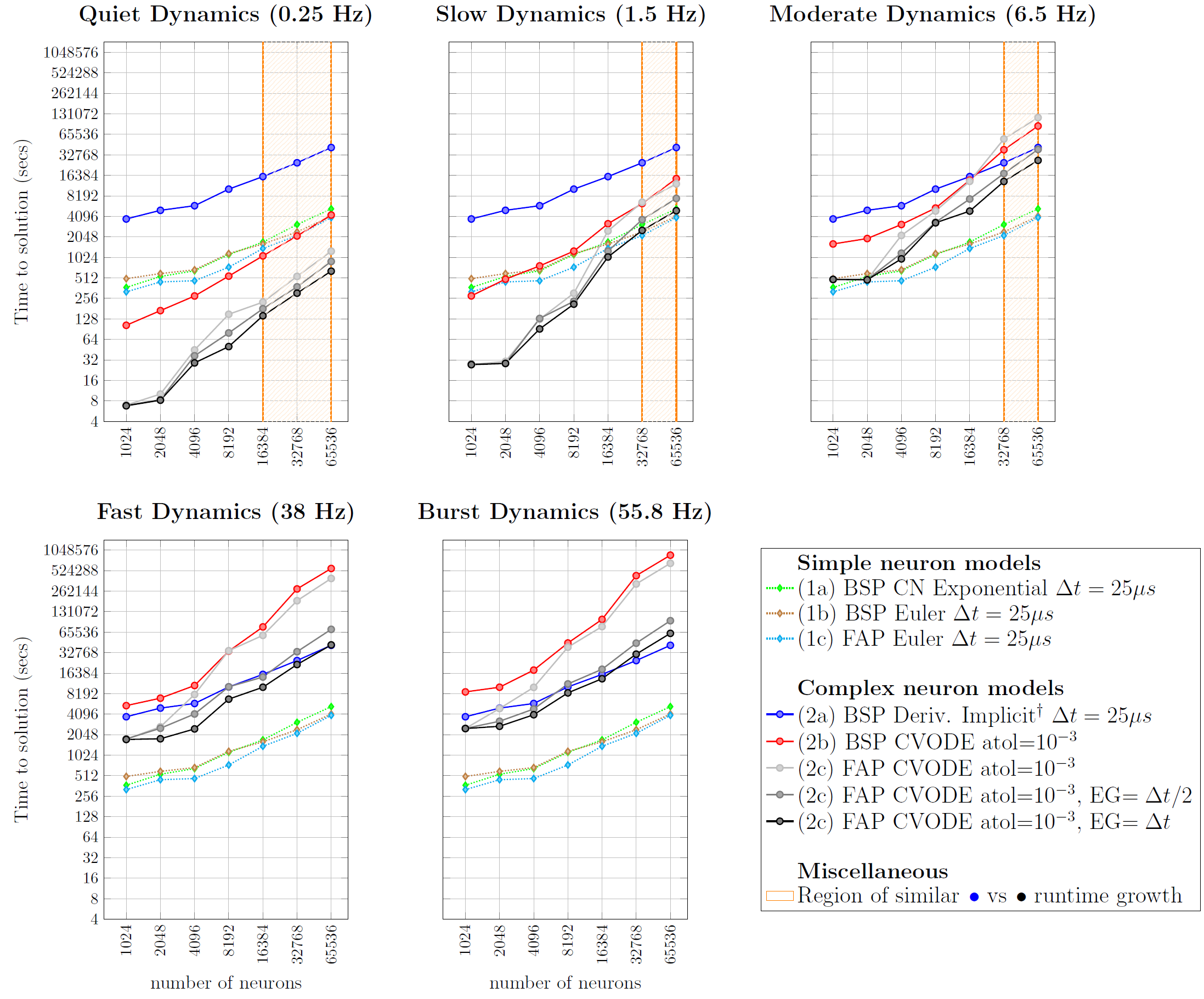
Quoting the previous paper: “Fixed step methods do not yield significantly-different execution times across different spiking regimes. This is due to the homogeneous computation of neuron state updates throughout time, and the light computation attached to synaptic events and collective communication not yielding a substantial increase of runtime. The difference in execution times measured across the five regimes was of about \(2\%\), which we consider negligible. On the other hand, as expected, variable step executions are penalized on regimes with high discontinuity rates. It is noticeable that the runtimes of fixed- and variable-step solvers approximate as we increase the spiking rate, i.e. the increase of runtimes with the input size is steeper for variable timestep (2b\(\hspace{0.3mm}{\color{red!80}\bullet}\) and 2c\(\hspace{0.3mm}{\color{black}\bullet}{\color{gray}\bullet}{\color{lightgray}\bullet}\)) compared to fixed timestep methods (2a\(\hspace{0.3mm}{\color{blue!80}\bullet}\)). This is due to discontinuities in variable-step being delivered throughout a continuous time line, compared to the discrete delivery instants of the fixed-step methods — therefore increase the number of interpolation steps; and the iterative model of the variable timestep reinitializing the state computation with small step sizes on each IVP reset, compared to the constant-sized step of fixed step methods. A remarkable performance is visible on the quiet dynamics use case, where our fully-implicit ODE solver of complex models (with Newton iterations), still runs faster than the simple solver resolving only a system of linear equations. The underlying rationale is that — despite the inherent computation cost of Newton iterations in the variable step methods — the low level of discontinuities allow for very long steps, that surpass the simulation throughput of simple solvers running on fixed step methods.”
For further details, detailed comparisons on the performance of Variable Step Event Grouping, Fully-Asynchronous vs Bulk-Synchonous Execution Models, Runtime Dependency on Input Size and Spike Activity, and the Overall Runtime Speed-up Estimation of 228.5-24.6x (based on the distribution of neurons per spiking regime on the brain), refer to the article preprint.