Variational Autoencoders (VAEs) and Generative Adversarial Neural Networks (GANs)
In our quest for understanding generative models in Machine Learning, we started by learning Statistics for ML Engineers, then we looked at Bayesian Linear Regression and the Exponential Family of Distributions to learn how to compute the Maximum Likelihood (MLE) and Maximum a Posteriori (MAP) estimators on parametric distributions. We then looked into Variational Inference as a method to perform generative ML on non-parametric or computationally-intractable Bayesian formulations. In this post, we continue our quest, and look at two new methods for non-parametric distributions based on neural networks: Variational Autoencoders (VAEs) and Generative Adversatial Neural Network (GANs).
Variational Autoencoder (VAE)
credit: most content in this post is a summary of the papers Auto-Encoding Variational Bayes and An Introduction to Variational Autoencoders from Diederik P. Kingma, Max Welling at the Uversiteit van Amsterdam.
The papers introduces Variational Autoencoders, aiming at performing efficient inference and learning in probabilistic models whose latent variables and parameters have intractable posterior distributions, and on large datasets. The SGVB (Stochastic Gradient Variational Bayes) estimator presented can be used for efficient approximation of posterior inference in almost any model with continuous latent variables, and because it’s differentiable, it can be optimized with e.g. gradient descent. The AutoEncoding Variational Bayes (AEVB) algorithm presented uses the SGVB estimator to optimize a model that does efficient approximate posterior inference using simple sampling (from parametric distributions).
The VAE is a probabilistic auto-encoder, where the probabilistic encoder (aka recognition model) and decoder (aka generative model) are represented as neural networks. The AEVB algorithm is a learning/inference algorithm that can be used to find the parameters of the VAE, i.e. to perform approximate variational inference in the directed graphical model of the VAE.
Input datapoints \(x\) are generated as following:
- a value \(z(i)\) is generated from some prior distribution \(p_{\theta^*}(z)\); and
- a value \(x(i)\) is generated from the likelihood distribution \(p_{\theta^∗}(x \mid z)\).
The assumptions are that both the prior and likelihood functions are parametric differentiable distributions, and that \(\theta^*\) and \(z(i)\) are unknown. There’s also the assumption of intractability as in:
- the integral of the evidence or marginal likelihood \(\int p_\theta(z) p\theta(x \mid z) dz\) is intractable;
- the true posterior density \(p\theta (z \mid x)\) is intractable, so the expectation maximization algorithm cant be used; and
- the algorithms for any mean-field approximation algorithm are also intractable. This is the level of intractability common to DNNs with nonlinear hidden layers.
The paper propose solutions to an efficient approximation of MAP estimation of parameters \(\theta\), of the posterior inference of the latent variable \(z\) and the marginal inference of the variable \(x\). Similarly to other variational inference methods, the intractable true posterior \(p_{\theta}(z \mid x)\) is approximated by \(q_\phi(z \mid x)\) (the Encoder), whose parameters \(\phi\) are not computed by a closed-form expectation but by the Encoder DNN instead. \(p_\theta(x \mid z)\) is the Decoder, that given a \(z\) will produce/generate the output which is a distribution over the possible values of x. Given a datapoint \(x\) the encoder produces produces a distribution (e.g. a Gaussian) over the possible values of the code \(z\) from which the datapoint \(x\) could have been generated.
Non-Variational vs Variational AutoEncoders
The VAE proposed includes a DNN decoder, a DNN decoder, with parameters \(\theta\) and \(\phi\) optimized together with the AEVB algorithm, where \(p_\theta(x \mid z)\) is a Gaussian/Bernoulli with distribution parameters computed from \(z\). Therefore the VAE can be viewed as two coupled, independent parameterized models: the encoder/recognition models, and the decoder/generative model (trained together), where the encoder delivers to the decoder an approximation to its posterior over latente random variables.
The difference between Variational Autoencoders and regular Autoencoders (such as sequence-to-sequence encoder-decoder) is that:
- in regular AEs the latent representation of \(z\) is both the output of the encoder and input of the decoder;
- in VAEs the output of the decoder are the parameters of the distributions of \(z\) – e.g. mean and variance in case of a Gaussian distribution – and \(z\) is drawn from those parameters and then passed to the decoder;
In practice, they can be vizualised as:
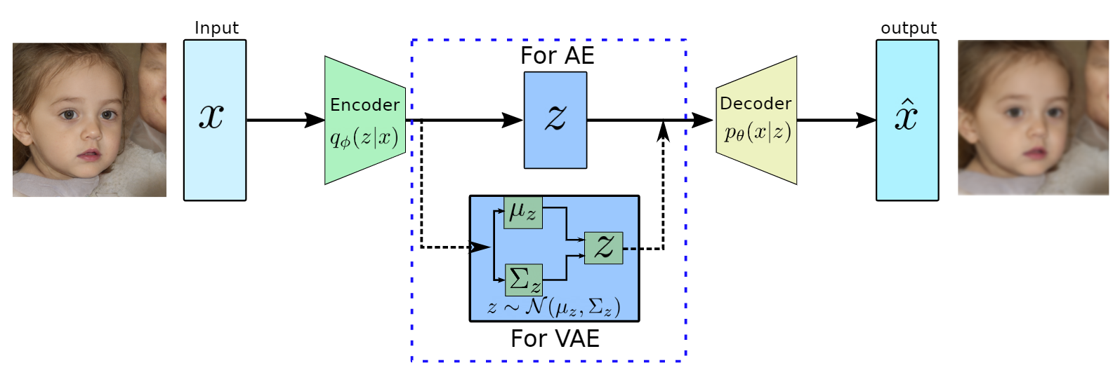
VAE vs AE structure (image credit: Variational Autoencoders, Data Science Blog, by Sunil Yadav))
Why VAE instead of Variational Inference
One advantage of the VAE framework, relative to ordinary Variational Inference, is that the encoder is now a stochastic function of the input variables, in contrast to VI where each data-case has a separate variational distribution, which is inefficient for large datasets.
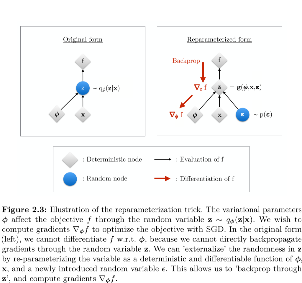
The reparametrization Trick
The authors noticed that the sampling induces sampling noise in the gradients required for learning (or that because \(z\) is randomly generated and cannot be back-propagated). In practice, randomness disrupts the deterministic computation of gradients, making it impossible to directly optimize the model via gradient descent. To counteract that, they authors propose the “reparameterization trick”.
The reparameterization trick decouples the sampling process from the stochasticity by introducing a deterministic transformation. Instead of sampling from \(z \sim N(\mu, \sigma^2)\), we rewrite \(z = \mu + \sigma \cdot \epsilon\), where \(\epsilon\) is the standard gaussian ie \(\epsilon \sim N(0,1)\).
Why does this work:
- The randomness is now isolated in \(𝜖\), which does not depend on the model parameters.
- The computation of \(𝑧\) becomes a differentiable function of \(𝜇\) and \(𝜎\), allowing gradients to flow through \(𝜇\) and \(𝜎\) during backpropagation, because the transformation \(𝑧 = 𝜇 + 𝜎 ⋅ 𝜖\) is fully differentiable with respect to these parameters.
The loss function
The loss function is a sum of two terms:

The first term is the reconstruction loss (or expected negative log-likelihood of the i-th datapoint). The expectation is taken with respect to the encoder’s distribution over the representations, encouraging the VAE to generate valid datapoints. This loss compares the model output with the model input and can be the losses we used in regular autoencoders, such as L2 loss, cross-entropy, etc.
The second term is the Kullback-Leibler divergence between the encoder’s distribution \(q_{\theta}(z \mid x)\) and the standard Gaussians \(p(z)\), where \(p(z)=\mathcal{N}(\mu=0, \sigma^2=1)\). This divergence compares the latent vector with a zero mean, unit variance Gaussian distribution, and penalizes the VAE if it starts to produce latent vectors that are not from the desired distribution. If the encoder outputs representations \(z\) that are different than those from a standard normal distribution, it will receive a penalty in the loss. This regularizer term means ‘keep the representations \(z\) of each digit sufficiently diverse’.
Results
The paper tested the VAE on the MNIST and Frey Face datasets and compared the variational lower bound and estimated marginal likelihood, demonstrating improved results over the wake-sleep algorithm.
Detour: why do we maximize the Expected Value?
In the Bayesian setup, it is common that the loss function is the sum of the expected values of several terms. Why?
It all goes down to the Law of large numbers. According to the law, the average of the outcomes of a large number of trials should be close to the expected value, and it tends to approximates the expected value as the number of trials increases.
Imagine we are playing a game (BlackJack, Slots, Rock-Paper-Scissors) that is repeatable as many times as desired. Because of the law of large numbers, we know that value of wins will over \(n\) iterations of the game will approximate \(n \mathbb{E}(X)\). In practice, we want to optimise our problem according to the most-likely outcome of our experiment, i.e. maximize its expected value;
So in practice, the law of large numbers will often guarantee a better outcome over the long run, and we maximize that outcome by maximizing the expected outcome of our optimisation in the long run.
Generative Adversarial Neural Network (GAN)
credit: most content in this post is a summary of the paper Generative Adversarial Networks, published at NeurIPS 2014, by Ian Goodfellow and colleagues at the Unviersity of Montreal.
The paper introduces a new generative model composed of two models trained simultaneously:
- a generative model G that captures the data distribution; and
- a discriminative model D that estimates the probability that a sample came from the training data rather than G;
The training procedure for G is to maximize the probability of D making a mistake. This framework is the minimax 2-player game. The adversarial framework comes from the fact that the generative model faces the discriminative model, that learns wether a sample is from the model distribution or from the data distribution. Quoting the authors: “The generative model can be thought of as analogous to a team of counterfeiters, trying to produce fake currency and use it without detection, while the discriminative model is analogous to the police, trying to detect the counterfeit currency. Competition in this game drives both teams to improve their methods until the counterfeits are indistiguishable from the genuine articles.”
Mathematical setup
The goal of the generative model is to generate samples by passing a random noise \(z\) through a multilayer perceptron.
- The generator \(G(z \mid \theta_g)\) is a multilayer perceptron with parameters \(\theta_g\).
- \(p_z(z)\) is the prior on the input noise variables.
- The generator \(G\) implicitly defines a probability distribution \(p_g\) as the distribution of the samples \(G(z)\) obtained when \(z \sim p_z\);
- The goal of the generator is to learn the distribution \(p_g\) over data \(x\), in order to fake it “well enough” and trick the discriminator;
The discriminative model is also a multilayer perceptron.
- The discriminator \(D(x \mid \theta_d)\) takes the input \(x\) and based on its DNN parameters \(\theta_d\) it outputs a single scalar representing the probability that \(x\) came from the data rather than \(p_g\);
The overall structure of the generator and discriminator training can be pictured as:
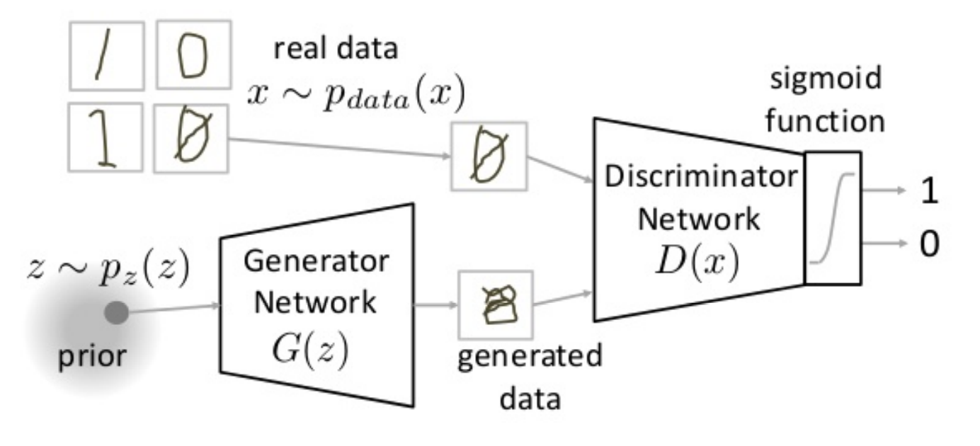
The GAN model (image credit: Benjamin Striner, lecture notes CMU 11-785)
Loss and minimax challenge
We train the discriminator \(D\) to best guess the source of the data, i.e. maximize the probability to assign the correct label to the training example and samples from \(G\).
We train the generator \(G\) simultaneously to minimize \(1-D((G(z)))\), i.e. be able to fake the data well enough. In practice, \(D\) and \(G\) are playing a two-player minimax game with value function \(V(G,D)\):

The loss function is a sum of two penalization terms:
- on the first term we optimise the discriminator, such that on the long run, we expect all real inputs (drawn from the data, ie \(x \sim p_{data}\)) to be as correct as possible;
- on the second term we optimise the discriminator and discriminator, such that on the long run, we expect all fake inputs (generated by the discriminator, ie \(z \sim p_z\)) to be also as correct as possible;
Finally, notice there is a \(log\) term added to both expected value terms. This is because the objective function is the product of multiple probabilities, in this case \(D(x) * (1-D(G(z)))\). Adding the \(log\) makes the optimisation return the same optima — as \(log\) is monotonic — while making it faster and more numerical stable. We also add the expectation term to the loss because we want to minimize the loss that we expect after several samples (law of large numbers). Thus:
\[\mathbb{E} \left[ log(D(x) * (1-D(G(z)))) \right] = \mathbb{E} \left[ log(D(x)) \right] + \mathbb{E} \left[ log(1-D(G(z))) \right]\]In section 4 (theoretical results) the authors show that indeed, when given enough capacity to the discriminator and generator, it is possible to retrieve the data generating distribution. In practice, it shows that this minimax game has a global optimum for \(p_g = p_{data}\), and therefore the loss function can be optimized.
Challenge: different convergence speed in the optimization of Generator and Discriminator
Because the objective function is much simpler, the discriminator trains much faster than the generator. To overcome it, training is performed by alternating between \(k\) steps of optimizing \(D\) and one step of optimizing \(G\). The underlying rationale is that “early in learning, when \(G\) is poor, \(D\) can reject samples with high confidence because they are clearly different from the training data. In this case, \(log(1 − D(G(z)))\) saturates.
Challenge: saturation of discriminator loss
The loss equation may not provide sufficient gradient for \(G\) to learn well. Early in learning, when \(G\) is poor, \(D\) can reject samples with high confidence because they are clearly different from the training data. In this case, \(log(1 − D(G(z)))\) saturates. Saturation means it’s not updating . Which means it is on some kind of a local minimum rather than in the desired global minima. In practice this means that this term of the loss function will not provide any signal (gradients) for the update of the loss, making it useless. I.e. when the discriminator performs significantly better than the generator, the updates to the discriminator are either inaccurate, or disappear.
This leads to two main problems:
- mathematically, the update of the parameters is none or very small, so the stepping in the loss landscape is very slow;
- computationally, arithmetic operations over very small values lead to incorrect (or “always zero”) results due to insufficient floating point precision in the processor (typically 16 or 32 bits);
The work around suggested by the authors is to change the algorithm for training the generator, and instead of minimizing \(\log(1 − D(G(z)))\), they maximize \(\log D(G(z))\) so that the optimisation landscape “provides much stronger gradients early in training”. See the pseudocode at the end of this post for a clearer explanation.
Challenge: Mode collapse
This challenge was not part of the original publication, and it was not discovered until later. In a regular scenario, we want GANs to generate a range of outputs, or ideally, a new random valid output for every random input to the generator. Instead, it may happen that sometimes we have a monotonous output, i.e. a range of very similar outputs. This phenomenon is called Mode Collapse and is detailled in this paper as: “This event occurs when the model can only fit a few modes of the data distribution, while ignoring the majority of them”. In this article they propose a workaround using second-order gradient information. However, this is a field of intense research and several solutions have been proposed, to name a few: a different loss function (Wasserstein loss), Unrolled GANs that incorporates current and future discriminator’s classification in the loss function (so that generator can’t over optimize for a single discriminator), Conditional GANs, VQ-VAEs, etc…
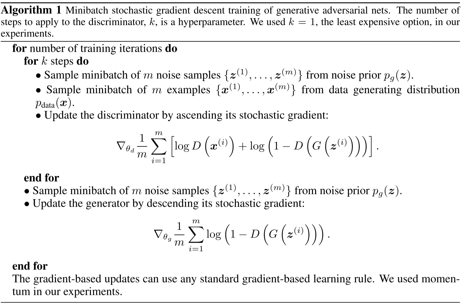
Training algorithm
This final training algorithm is the following: