Diffusion models (DDPM, DiT, Rectified Flow)
Similarly to generative adversarial networks (GANs) and variational autoencoders (VAEs), diffusion models are generative models that learn to convert noise from a distribution into a data sample, the denoising process. A diffusion model is made of two Markov chains: a forward process that gradually adds noise to the data, and a learnable reverse process that removes the noise one step at a time, with one pass of a neural network per step. The transitions of the reverse chain are learned with variational inference, and, once the model is trained, a sampling algorithm generates new data from pure noise.
The following picture illustrates both chains: the reverse process (solid arrows) turns noise into an image, and the forward process (dashed arrow) adds noise to it:

Adapted from: Denoising Diffusion Probabilistic Models.
Forward process
The forward diffusion process \(q\) of Denoising Diffusion Probabilistic Models (DDPM) is a Markov chain of \(T\) steps, where each step adds Gaussian noise to the output of the previous step, according to a variance \(\beta_t \in (0,1)\) for each of the \(T\) timesteps, typically with \(0 \lt \beta_1 \lt \beta_2 \lt \dots \lt \beta_T \lt 1\). \(\beta_t\) can be learned or (in this case) fixed as a hyper-parameter. The process starts with the data as \(\mathbf{x}_0\) for \(t=0\) and gradually samples and adds Gaussian noise at each step, producing noisy samples \(\mathbf{x}_1, ..., \mathbf{x}_T\). The timestep \(t\) is the time of the process, by analogy with diffusion in physics, e.g. of a drop of ink that spreads in water over time until the color is uniform. Similarly, \(\mathbf{x}_t\) holds more noise and less of the data as time goes on, and the reverse process goes back in time, from the noise to the data. The timesteps are equally spaced in time, but each one adds noise of a larger variance \(\beta_t\) than the one before. The forward process \(q\) is then represented as (Eq. 2 in the paper):
\[q(\mathbf{x}_t \vert \mathbf{x}_{t-1}) = \mathcal{N}(\mathbf{x}_t; \sqrt{1 - \beta_t} \mathbf{x}_{t-1}, \beta_t\mathbf{I}) \quad\]i.e. each new sample \(\mathbf{x}_t\) is drawn from a Gaussian distribution with mean \(\sqrt{1-\beta_t} \mathbf{x}_{t-1}\) and covariance \(\beta_t\mathbf{I}\) (each dimension gets independent noise of variance \(\beta_t\)). With \(\alpha_t = 1 - \beta_t\), sampling from it is equivalent to sampling \(\epsilon \sim \mathcal{N}(0, \mathbf{I})\) and then setting \(\mathbf{x}_t = \sqrt{\alpha_t} \mathbf{x}_{t-1} + \sqrt{1-\alpha_t}\epsilon\).
Another property of the forward process, noted in the paper, is that \(\mathbf{x}_t\) can be sampled at any time \(t\) conditioned directly on \(\mathbf{x}_0\), instead of on \(\mathbf{x}_{t-1}\) (i.e. iteratively). This is because the sum of independent Gaussian random variables is also a Gaussian random variable, whose variance is the sum of their variances. Expanding \(\mathbf{x}_{t-1}\) with the same formula gives \(\mathbf{x}_t = \sqrt{\alpha_t \alpha_{t-1}} \mathbf{x}_{t-2}\) plus two independent noises of variances \(\alpha_t (1-\alpha_{t-1})\) and \(1-\alpha_t\), i.e. a single noise of variance \(1-\alpha_t \alpha_{t-1}\). Repeating this down to \(\mathbf{x}_0\), the forward process can also be written as (Eq. 4 in the paper):
\[q (\mathbf{x}_t \mid \mathbf{x}_0) = \mathcal{N} (\mathbf{x}_t ; \sqrt{\bar{\alpha}_t} \mathbf{x}_0, (1-\bar{\alpha}_t) \mathbf{I})\]where \(\bar{\alpha}_t = \prod_{s=1}^t \alpha_s\). Equivalently, \(\mathbf{x}_t = \sqrt{\bar{\alpha}_t} \mathbf{x}_0 + \sqrt{1-\bar{\alpha}_t} \epsilon\), with \(\epsilon \sim \mathcal{N}(0, \mathbf{I})\).
The implementation starts by defining \(\beta_t\), \(\alpha_t\) and \(\bar{\alpha}_t\). There are many \(\beta_t\) variance schedulers, but for simplicity, the implementation uses a linear scheduler for \(\beta_t\).
Note that Eq. 4 also tells how much of the signal \(\mathbf{x}_0\) is left at the last step: \(\mathbf{x}_T\) is close to pure noise \(\mathcal{N}(0, \mathbf{I})\) only if \(\bar{\alpha}_T \approx 0\). The paper uses \(T=1000\) steps and a \(\beta_t\) that increases linearly from \(\beta_1=10^{-4}\) to \(\beta_T=0.02\), leading to \(\sqrt{\bar{\alpha}_T} \approx 0.006\).
To sample faster, the implementation uses \(T=100\) steps instead. Unlike the original DDPM code, and as in the code of Improved DDPM, it scales \(\beta_1\) and \(\beta_T\) by \(1000/T\), so that \(\mathbf{x}_T\) is still close to pure noise:
    T = 100 # the paper uses T=1000
    β_1, β_T = 0.0001 * 1000 / T, 0.02 * 1000 / T # the paper's values, scaled by 1000/T
    # arrays are 0-indexed: index i holds the value of the paper's timestep t=i+1
    β = torch.linspace(β_1, β_T, T, device=device)
    α = 1. - β
    α_cumprod = torch.cumprod(α, axis=0)
Now the forward process \(q (\mathbf{x}_t \mid \mathbf{x}_0)\) of Eq. 4 is defined as:
    @torch.no_grad()
    def q_sample(x_0, t, noise):
        """ Eq. 4: sample x_t from x_0, by scaling and shifting a noise sampled from N(0, I) """
        sqrt_α_cumprod_t = torch.sqrt(α_cumprod[t])[:, None, None, None]
        sqrt_1_minus_α_cumprod_t = torch.sqrt(1. - α_cumprod[t])[:, None, None, None]
        return sqrt_α_cumprod_t * x_0 + sqrt_1_minus_α_cumprod_t * noise
And that is all the forward process needs: it has no learned parameters, and q_sample takes an image to any step \(t\) in one operation. The model is learned in the reverse process, which turns the noise back into data.
Reverse process
The reverse process is a Markov chain \(p_\theta(\mathbf{x}_{0:T})\) with learned Gaussian transitions starting at \(p(\mathbf{x}_T) = \mathcal{N} (\mathbf{x}_T ; 0, \mathbf{I})\), and:
\[p_\theta(\mathbf{x}_{t-1} \vert \mathbf{x}_t) = \mathcal{N}(\mathbf{x}_{t-1}; \mu_\theta(\mathbf{x}_t, t), \Sigma_\theta(\mathbf{x}_t, t) )\]The distribution of the true denoising step \(q(\mathbf{x}_{t-1} \mid \mathbf{x}_t)\) is not known, as it depends on the whole data distribution, so it is approximated with \(p_{\theta}\), parameterized by a neural network. This is where variational inference comes in. This distribution will be approximated to a Gaussian distribution, with a learnable mean \(\mu_\theta\) and covariance \(\Sigma_\theta\) (Eq. 1 in the paper). This is a good approximation when the \(\beta_t\) are small, as the reverse of a small Gaussian diffusion step is also (approximately) Gaussian. The training maximizes the evidence lower bound (ELBO) on the log-likelihood of the data \(\mathbf{x}_0\), i.e. it minimizes the variational bound \(L\) on its negative log-likelihood (Eq. 3 in the paper):
\[\mathbb{E} \left[ - \log p_\theta(\mathbf{x}_0) \right] \le \mathbb{E}_q \left[ - \log \frac{p_\theta(\mathbf{x}_{0:T})}{q(\mathbf{x}_{1:T} \vert \mathbf{x}_0)} \right] =: L\]Taking the log turns the products over the steps of both chains into sums, and, with Bayes’ rule, \(L\) can be rewritten as one term per step (Eq. 5 in the paper, derived in its Appendix A):
\[L = \mathbb{E}_q \bigg[ \underbrace{\text{KL}(q(\mathbf{x}_T \vert \mathbf{x}_0) \parallel p(\mathbf{x}_T))}_{L_T} + \sum_{t > 1} \underbrace{\text{KL}(q(\mathbf{x}_{t-1} \vert \mathbf{x}_t, \mathbf{x}_0) \parallel p_\theta(\mathbf{x}_{t-1} \vert \mathbf{x}_t))}_{L_{t-1}} \underbrace{- \log p_\theta(\mathbf{x}_0 \vert \mathbf{x}_1)}_{L_0} \bigg]\]where KL is the Kullback-Leibler divergence, \(L_T\) has no learnable parameters (it is a constant), and \(L_0\) is the reconstruction term of the last denoising step. Each term \(L_{t-1}\) compares a reverse step with the true denoising step, which becomes tractable when it is also conditioned on the data \(\mathbf{x}_0\). This forward process posterior is given by (Eq. 6 in the paper):
\[q(\mathbf{x}_{t-1} \mid \mathbf{x}_t, \mathbf{x}_0 ) = \mathcal{N} (\mathbf{x}_{t-1} ; \tilde{\mu}_t (\mathbf{x}_t, \mathbf{x}_0), \, \tilde{\beta}_t \mathbf{I})\]where the posterior variance \(\tilde{\beta}_t = \frac{1-\bar{\alpha}_{t-1}}{1-\bar{\alpha}_t} \beta_t\) is a constant that depends only on the noise schedule, and the posterior mean is computed as (Eq. 7 in the paper):
\[\tilde{\mu}_t(\mathbf{x}_t, \mathbf{x}_0) = \frac{\sqrt{\bar{\alpha}_{t-1}} \beta_t }{1-\bar{\alpha}_t} \mathbf{x}_0 + \frac{\sqrt{\alpha_t}(1-\bar{\alpha}_{t-1})}{1-\bar{\alpha}_t} \mathbf{x}_t\]In the original paper, the variance of \(p_\theta\) is not learned: it is set to \(\Sigma_\theta(\mathbf{x}_t, t) = \sigma^2_t \mathbf{I}\), with \(\sigma^2_t = \beta_t\) or \(\sigma^2_t = \tilde{\beta}_t\) (both gave similar results). Improved DDPM later learned it, as an interpolation between \(\beta_t\) and \(\tilde{\beta}_t\) trained with the bound \(L\), which improves the log-likelihood and allows sampling with fewer steps. The diffusion transformer (DiT) learns it the same way. However, the variance only sets the noise that a stochastic sampler adds at each step, while current models sample with deterministic solvers (see flow matching), so they rarely learn it.
With fixed variances, the KL divergence \(L_{t-1}\) between the posterior and \(p_\theta\) reduces to the squared distance between their means (Eq. 8 in the paper):
\[L_{t-1} = \mathbb{E}_q \left[ \frac{1}{2 \sigma_t^2} \| \tilde{\mu}_t(\mathbf{x}_t, \mathbf{x}_0) - \mu_\theta(\mathbf{x}_t, t) \|^2 \right] + C\]where \(C\) is a constant that does not depend on \(\theta\). So the most straightforward parameterization is a model \(\mu_\theta\) that predicts the posterior mean \(\tilde{\mu}_t\). However, replacing \(\mathbf{x}_0 = \frac{1}{\sqrt{\bar{\alpha}_t}} \left( \mathbf{x}_t - \sqrt{1-\bar{\alpha}_t} \epsilon \right)\) (Eq. 4) in Eq. 7, the posterior mean is given by (Eqs. 9 and 10 in the paper):
\[\tilde{\mu}_t(\mathbf{x}_t, \mathbf{x}_0) = \frac{1}{\sqrt{\alpha_t}} \left( \mathbf{x}_t - \frac{\beta_t}{\sqrt{1-\bar{\alpha}_t}} \epsilon \right)\]So \(\mu_\theta\) must predict this mean given \(\mathbf{x}_t\). As \(\mathbf{x}_t\) is already an input to the model, the authors propose a parameterization where the model predicts the noise \(\epsilon_\theta(\mathbf{x}_t, t)\) at step \(t\) instead of the mean \(\mu_\theta(\mathbf{x}_t, t)\). (Section 3.2) The mean can then be computed as (Eq. 11 in the paper):
\[\mu_\theta(\mathbf{x}_t, t) = \frac{1}{\sqrt{\alpha_t}} \left( \mathbf{x}_t - \frac{\beta_t}{\sqrt{1-\bar{\alpha}_t}} \epsilon_\theta(\mathbf{x}_t, t) \right)\]where the model \(\epsilon_\theta(\mathbf{x}_t, t)\) takes as input the image \(\mathbf{x}_t\) sampled at the timestep \(t\), and also the timestep \(t\), which the model receives as a timestep embedding. This is then coded as:
    def eq11_μ_θ(x_t, ε_θ, t):
        """ Eq. 11: the mean of the reverse step, from the noise ε_θ predicted by the model """
        α_t, β_t, α_cumprod_t = α[t][:, None, None, None], β[t][:, None, None, None], α_cumprod[t][:, None, None, None]
        return (x_t - β_t * ε_θ / torch.sqrt(1. - α_cumprod_t)) / torch.sqrt(α_t)
Replacing both means of Eq. 8 by Eqs. 10 and 11, each term \(L_{t-1}\) becomes a weighted mean squared error between the sampled and the predicted noise (Eq. 12 in the paper):
\[L_{t-1} - C = \mathbb{E}_{\mathbf{x}_0, \epsilon} \left[ \frac{\beta_t^2}{2 \sigma_t^2 \alpha_t (1-\bar{\alpha}_t)} \| \epsilon - \epsilon_\theta(\sqrt{\bar{\alpha}_t} \mathbf{x}_0 + \sqrt{1-\bar{\alpha}_t} \epsilon, t) \|^2 \right]\]As a loss function, the implementation follows the paper and drops the weights, i.e. it uses a simple mean squared error (Eq. 14) between the sampled noise \(\epsilon\) and the predicted noise \(\epsilon_\theta\) (the Huber loss and the mean absolute error are also popular choices):
\[\mathcal{L}_\text{simple}(\theta) = \mathop{\mathbb{E}}_{t, \mathbf{x}_0, \epsilon} \left[ \| \epsilon - \epsilon_\theta(\sqrt{\bar{\alpha}_t} \mathbf{x}_0 + \sqrt{1-\bar{\alpha}_t} \epsilon, t)\| ^2 \right]\]where \(t\) is sampled uniformly between \(1\) and \(T\). So \(\mathcal{L}_\text{simple}\) is a simplified version of the bound \(L\): the authors found it to be simpler to implement and to yield better sample quality.
Flow matching
In DDPM, the input \(\mathbf{x}_t\) of the network mixes the data and the noise with the coefficients \(\sqrt{\bar{\alpha}_t}\) and \(\sqrt{1-\bar{\alpha}_t}\), so the noisy sample moves on a curved path between them, and the sampler needs many steps to follow it. Flow matching trains the network to predict the velocity of the sample along a chosen path, with a regression loss that needs no variational bound. The path is the curve that \(\mathbf{x}_t\) follows from the data sample \(\mathbf{x}_0\) to the noise sample \(\epsilon\), and it is chosen with the coefficients of \(\mathbf{x}_0\) and \(\epsilon\) in \(\mathbf{x}_t\). The rectified flow chooses the straight line between the data and the noise, with a continuous time \(t \in [0, 1]\), and its loss is given by:
\[\mathbf{x}_t = (1-t)\, \mathbf{x}_0 + t\, \epsilon, \quad \mathcal{L}_\text{FM}(\theta) = \mathop{\mathbb{E}}_{t, \mathbf{x}_0, \epsilon} \left[ \| (\epsilon - \mathbf{x}_0) - v_\theta(\mathbf{x}_t, t) \|^2 \right]\]where the network \(v_\theta\) learns a vector field, i.e. a velocity for every point \(\mathbf{x}_t\) at every time \(t\), and \(\epsilon - \mathbf{x}_0\) is the velocity \(d\mathbf{x}_t / dt\) of the sample. Compared with \(\mathcal{L}_\text{simple}\), only the input and the target change, so the same network trains with either loss. The following picture illustrates both paths for one sample, and the coefficients of the data and the noise along them:
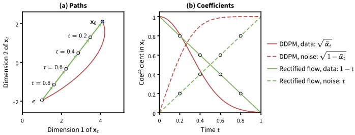
Paths of the noisy sample \(\mathbf{x}_t\) from a data sample \(\mathbf{x}_0\) to a noise sample \(\epsilon\); for DDPM, \(t\) is the step divided by \(T\). (a) DDPM (red) moves on a curve, and the rectified flow (green) on a straight line, which 5 Euler steps (arrows) of \(\Delta t = 0.2\) follow exactly. (b) The coefficients of \(\mathbf{x}_0\) and \(\epsilon\) in \(\mathbf{x}_t\); the dots mark the steps of (a).
The implementation keeps the \(T\) timesteps of DDPM, sampled uniformly, so that the network embeds the time as before: the 0-indexed timestep t of the code is the time \((t+1)/T\), from \(1/T\) to \(1\). The straight path is then computed as:
    @torch.no_grad()
    def fm_interpolate(x_0, t, noise):
        """ flow matching: the straight path x_t = (1-t) x_0 + t ε, at the time (t+1)/T of the 0-indexed step t """
        t = ((t + 1) / T)[:, None, None, None]
        return (1 - t) * x_0 + t * noise
The velocity is easy to predict near both ends, where the input is almost the data or almost the noise, and hardest in the middle. So Scaling Rectified Flow Transformers for High-Resolution Image Synthesis samples \(t\) from a logit-normal distribution instead of a uniform one, i.e. \(t = 1/(1+e^{-u})\) with \(u \sim \mathcal{N}(m, s^2)\), which trains more on the middle timesteps. Of all the formulations that the paper compares, the rectified flow with \(m = 0\) and \(s = 1\) ranks best on average.
Sampling solves the ordinary differential equation (ODE) \(d\mathbf{x}_t / dt = v_\theta(\mathbf{x}_t, t)\) of the learned vector field, from the noise at \(t = 1\) back to \(t = 0\). From each noise sample, the solution is a path that ends at one data sample, like the paths of the trained models in the pictures below. The simplest solver takes explicit (forward) Euler steps backward in time, \(\mathbf{x}_{t - \Delta t} = \mathbf{x}_t - \Delta t \, v_\theta(\mathbf{x}_t, t)\). Each step reads the velocity at the current point, so, unlike an implicit Euler step, it solves no equation.
Gradient descent (GD) with a fixed step size also takes explicit Euler steps, on the gradient flow \(d\theta / d\tau = -\nabla \mathcal{L}(\theta)\) of a loss \(\mathcal{L}\) over the optimization time \(\tau\). However, the field of GD is fixed, and GD runs until it reaches a minimum. The velocity of the sampler changes with \(t\), so the sampler descends no single loss: it runs for a fixed time, from \(t = 1\) to \(t = 0\), and ends wherever its path is at \(t = 0\). Gradient ascent on a fixed density of the data would instead send every sample to a mode, with no diversity.
The sampler adds no noise, and as its paths are straighter than the ones of DDPM, it needs fewer steps. However, the paths that the model learns are not fully straight: the straight lines between random pairs of noise and data cross each other, and the network predicts the average of their velocities where they cross. Reflow retrains the model on pairs of noise and the sample that the model generates from it. As these pairs come from paths that do not cross, the lines between them cross much less, and the new paths are nearly straight, so that one or a few steps suffice. The following picture illustrates these paths, for models trained on two-dimensional data with two clusters:
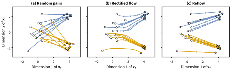
Paths from noise (white) to data (colored by cluster), with dots at the times \(0.75\), \(0.5\) and \(0.25\). (a) The lines between random pairs cross. (b) The paths of the trained model do not cross, but bend. (c) After reflow, they are nearly straight, with evenly spaced dots. Inspired by: Flow Straight and Fast: Learning to Generate and Transfer Data with Rectified Flow
With Gaussian noise, flow matching and diffusion are two parameterizations of the same model. The straight path is a noise schedule that scales the data by \(1-t\) and the noise by \(t\), instead of \(\sqrt{\bar{\alpha}_t}\) and \(\sqrt{1-\bar{\alpha}_t}\). The velocity is a combination of the predicted noise and data, and the sampler of Denoising Diffusion Implicit Models (DDIM), which uses a model trained as in DDPM but adds no noise, is the Euler sampler above on this schedule. So flow matching improves diffusion with its schedule, its target and the weighting of its loss over time, not with a new kind of model. These choices made it the training objective of most current image and video DiTs.
Diffusion transformers
As Transformers became a key building block of sequence-based ML, the 2022 paper Scalable Diffusion Models with Transformers introduced diffusion transformers. The paper is based on Vision Transformers (ViTs), which operate on patches of images. The DiT architecture is illustrated in the following picture:
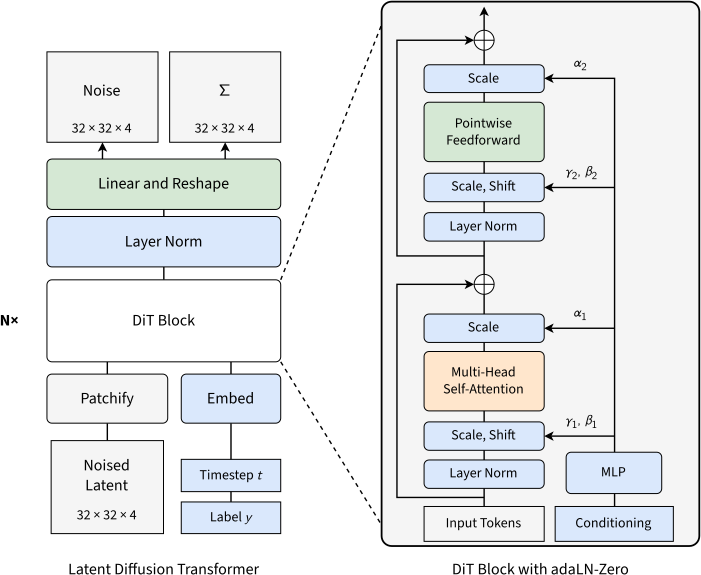
The Diffusion Transformer (DiT) architecture. Left: a conditional DiT on the pixels of the image; the noised image is decomposed into patches, embedded as tokens, processed by several DiT blocks and decoded into the patches of the noise (of the velocity, with flow matching). Right: the DiT block that adds the conditioning by adaptive layer norm (adaLN-Zero). The paper also tested in-context conditioning, cross-attention and adaLN blocks, and adaLN-Zero worked best. Inspired by: Scalable Diffusion Models with Transformers.
A conditional diffusion model takes extra information \(y\) as input, such as a class label, a text or an image, and its reverse process becomes \(p_\theta(\mathbf{x}_{t-1} \mid \mathbf{x}_t, y)\). In the adaLN-Zero architecture shown in the diagram, adaptive layer normalization is used to condition the model dynamically: instead of learning the scale \(\gamma\) and shift \(\beta\) parameters of each layer norm directly, these are regressed by a multilayer perceptron (MLP) from the sum of the embeddings of the timestep \(t\) and the class label \(y\) (the conditioning inputs). adaLN-Zero additionally regresses dimension-wise scaling parameters \(\alpha\) that are applied right before each residual connection, and initializes them to zero, so that each DiT block starts as the identity function. Note that these \(\alpha\) and \(\beta\) are unrelated to the \(\alpha_t\) and \(\beta_t\) of the noise schedule.
First, the DiT block regresses \(\gamma_1, \beta_1, \alpha_1, \gamma_2, \beta_2, \alpha_2\) from the conditioning c, and applies them around the attention and the feed-forward network, as in the picture. As in the official implementation, the output of a layer norm is scaled by \(1+\gamma\), so that \(\gamma = 0\) keeps it unchanged. The attention uses PyTorch’s scaled_dot_product_attention, which runs a fused kernel, such as FlashAttention, when the hardware supports it:
class DiTBlock(nn.Module):
    """ A DiT block with adaLN-Zero: self-attention and a feed-forward network, conditioned on c """

    def __init__(self, n_embd, n_heads=8, d_head=128, dropout_p=0.1):
        super().__init__()
        self.n_heads, self.dropout_p = n_heads, dropout_p
        self.ln1 = nn.LayerNorm(n_embd, elementwise_affine=False) # no learned scale and shift, adaLN regresses them
        self.query, self.key, self.value = [nn.Linear(n_embd, n_heads*d_head) for _ in range(3)] # projections of all heads
        self.out = nn.Sequential(nn.Linear(n_heads*d_head, n_embd), nn.Dropout(dropout_p)) # output projection
        self.ln2 = nn.LayerNorm(n_embd, elementwise_affine=False)
        self.ffw = nn.Sequential(nn.Linear(n_embd, 4*n_embd), nn.ReLU(), nn.Linear(4*n_embd, n_embd), nn.Dropout(dropout_p))
        self.adaLN = nn.Sequential(nn.SiLU(), nn.Linear(n_embd, 6*n_embd)) # MLP that regresses γ1, β1, α1, γ2, β2, α2
        nn.init.zeros_(self.adaLN[1].weight) # adaLN-Zero: α=0, so that the block starts as the identity
        nn.init.zeros_(self.adaLN[1].bias)

    def mha(self, x):
        """ multi-head self-attention, without a causal mask """
        B, N, _ = x.shape
        split = lambda y: y.view(B, N, self.n_heads, -1).transpose(1, 2) # (B, N, H*D) -> (B, H, N, D)
        q, k, v = split(self.query(x)), split(self.key(x)), split(self.value(x))
        dropout_p = self.dropout_p if self.training else 0. # the functional API does not know about eval mode
        x = F.scaled_dot_product_attention(q, k, v, dropout_p=dropout_p) # softmax(QKᵀ/√D)V of each head, (B, H, N, D)
        return self.out(x.transpose(1, 2).reshape(B, N, -1)) # (B, N, H*D) -> (B, N, E)

    def forward(self, x, c):
        γ1, β1, α1, γ2, β2, α2 = self.adaLN(c).unsqueeze(1).chunk(6, dim=-1) # each (B, 1, E)
        x = x + α1 * self.mha(self.ln1(x) * (1 + γ1) + β1) # scale by 1+γ, so that γ=0 is the identity
        x = x + α2 * self.ffw(self.ln2(x) * (1 + γ2) + β2)
        return x
Then, the constructor of the model defines the embeddings, the DiT blocks and the decoder:
class DiT(nn.Module):
    """ A Diffusion Transformer (DiT) model that predicts the noise ε_θ, or the velocity v_θ of flow matching """

    def __init__(self, timesteps, num_channels, img_size, patch_size=4, n_embd=48, n_blocks=12, num_labels=None):
        super().__init__()
        assert img_size % patch_size == 0, "Image size must be divisible by patch size"
        self.patch_size = patch_size
        patch_dim = patch_size*patch_size*num_channels # values per image patch

        # patch embedding (a linear layer) and positional embeddings
        self.patch_embedding = nn.Linear(patch_dim, n_embd)
        self.pos_embedding = nn.Embedding((img_size//patch_size)**2, n_embd)

        # timestep and class embeddings, summed into the conditioning (class only for a class-conditional model)
        self.t_embedding = nn.Embedding(timesteps, n_embd)
        self.class_embedding = nn.Embedding(num_labels, n_embd) if num_labels else None

        # DiT blocks, and a decoder: an adaptive layer norm and a linear layer that decodes each token into a patch
        self.blocks = nn.ModuleList([DiTBlock(n_embd) for _ in range(n_blocks)])
        self.decoder_ln = nn.LayerNorm(n_embd, elementwise_affine=False)
        self.decoder_adaLN = nn.Sequential(nn.SiLU(), nn.Linear(n_embd, 2*n_embd)) # MLP that regresses γ and β
        self.decoder = nn.Linear(n_embd, patch_dim)
Next comes the boilerplate code that splits the input image into the patches used by the attention module, and that merges the patches back into a single image:
    def patchify(self, x):
        """ break images (B, C, H, W) into NH*NW patches of PH*PW*C values, (B, NH*NW, PH*PW*C) """
        B, C, H, W = x.shape
        x = x.unfold(2, self.patch_size, self.patch_size).unfold(3, self.patch_size, self.patch_size) # (B, C, NH, NW, PH, PW)

        # linearize patches and flatten their values
        _, _, NH, NW, PH, PW = x.shape
        x = x.permute(0, 2, 3, 4, 5, 1) # (B, NH, NW, PH, PW, C)
        x = x.reshape(B, NH*NW, PH*PW*C)
        return x, dict(B=B, C=C, H=H, W=W, NH=NH, NW=NW, PH=PH, PW=PW)

    def unpatchify(self, x, shapes):
        """ merge patches (B, NH*NW, PH*PW*C) back into images (B, C, H, W) = (B, C, NH*PH, NW*PW) """
        B, C, H, W, NH, NW, PH, PW = shapes.values()
        x = x.reshape(B, NH, NW, PH, PW, C).permute(0, 5, 1, 3, 2, 4) # (B, C, NH, PH, NW, PW)
        return x.reshape(B, C, H, W)
Finally, the forward pass embeds the patches, sums the timestep embedding and the class embedding into the conditioning c, and runs the DiT blocks and the decoder:
    def forward(self, x, t, label=None):
        x, shapes = self.patchify(x) # (B, C, H, W) -> (B, N, P), for N patches of P=PH*PW*C values
        positions = torch.arange(x.shape[1], device=x.device)
        x = self.patch_embedding(x) + self.pos_embedding(positions) # (B, N, E)
        c = self.t_embedding(t) # conditioning (B, E): the timestep embedding,
        if label is not None: # plus the class embedding
            c = c + self.class_embedding(label)
        for block in self.blocks:
            x = block(x, c)
        γ, β = self.decoder_adaLN(c).unsqueeze(1).chunk(2, dim=-1) # each (B, 1, E)
        x = self.decoder(self.decoder_ln(x) * (1 + γ) + β) # (B, N, E) -> (B, N, P)
        return self.unpatchify(x, shapes) # ε_θ or v_θ, (B, C, H, W)
Training algorithm
The final training algorithm can now be put together:
\[\begin{array}{l} \hline \textbf{Algorithm 1} \text{ Training} \\ \hline \text{1:} \;\; \textbf{repeat} \\ \text{2:} \quad\; \mathbf{x}_0 \sim q(\mathbf{x}_0) \\ \text{3:} \quad\; t \sim \mathrm{Uniform}(\{1, \ldots, T\}) \\ \text{4:} \quad\; \boldsymbol{\epsilon} \sim \mathcal{N}(\mathbf{0}, \mathbf{I}) \\ \text{5:} \quad\; \text{Take gradient descent step on} \\ \qquad\qquad\; \nabla_\theta \left\| \boldsymbol{\epsilon} - \boldsymbol{\epsilon}_\theta(\sqrt{\bar{\alpha}_t} \mathbf{x}_0 + \sqrt{1-\bar{\alpha}_t} \boldsymbol{\epsilon}, t) \right\|^2 \\ \text{6:} \;\; \textbf{until} \text{ converged} \\ \hline \end{array}\]The DiT model is trained on the CIFAR-10 dataset, which contains 32 × 32 RGB images of 10 classes. The batch size is set to 48 images (per GPU). The training also keeps an exponential moving average (EMA) of the model weights with a decay of \(0.9999\), as DDPM and DiT do, and the sampler uses these averaged weights. Each step computes the loss on random timesteps and random noise, so the weights keep moving around a good solution, and their average is more stable. Without the EMA, the quality of the samples varies a lot during training, and the samples show color shifts (Improved Techniques for Training Score-Based Generative Models).
With flow matching, the loop takes the straight path and the velocity as the input and the target of the network instead. At the end of every epoch, the EMA model generates and saves new images.
    # load dataset from the hub
    dataset = load_dataset("uoft-cs/cifar10", split='train')
    transform = lambda image: (pil_to_tensor(image)/255)*2-1 # normalize to [-1,1]
    images = [ transform(image) for image in dataset["img"]]
    batch_size, channels, img_size = 48, images[0].shape[0], images[0].shape[-1]
    sampler = DistributedSampler(images)
    dataloader = DataLoader(images, batch_size=batch_size, sampler=sampler, drop_last=True)

    # model and optimizers
    model = DiT(T, channels, img_size, patch_size=4, n_blocks=4).to(device=device)
    ema_decay = lambda n: ((1 + n) / (10 + n)).clamp(max=0.9999) # 0.9999 as in the paper, with a warmup as in diffusers
    ema = AveragedModel(model, avg_fn=lambda ema_p, p, n: ema_decay(n) * ema_p + (1 - ema_decay(n)) * p).eval()
    model = torch.nn.parallel.DistributedDataParallel(model, device_ids=[local_rank] if torch.cuda.is_available() else None)
    optimizer = Adam(model.parameters(), lr=2e-4)

    # training loop
    for epoch in range(20):
        sampler.set_epoch(epoch) # shuffle the data differently at every epoch
        for step, x_0 in enumerate(dataloader):
            x_0 = x_0.to(device=device)
            t = torch.randint(0, T, (batch_size,), device=device) # Algorithm 1, step 3 (0-indexed)
            noise = torch.randn_like(x_0) # step 4
            x_t, target = (fm_interpolate(x_0, t, noise), noise - x_0) if flow else (q_sample(x_0, t, noise), noise)
            loss = F.mse_loss(model(x_t, t), target) # step 5: the loss L_simple, or L_FM with flow matching
            loss.backward()
            optimizer.step()
            optimizer.zero_grad(set_to_none=True)
            ema.update_parameters(model.module)
            if dist.get_rank() == 0:
                print(f"epoch {epoch}, step {step} loss: {loss.item()}")

        # save images generated with the EMA model
        if dist.get_rank() == 0:
            results_folder = Path("./results")
            results_folder.mkdir(exist_ok = True)
            img = euler_sampling(ema, shape=x_0.shape) if flow else alg2_p_sampling(ema, shape=x_0.shape)
            img = (img + 1) * 0.5 # from [-1,1] to [0,1]
            save_image(img, str(results_folder / f'sample-{epoch}.png'), nrow = batch_size)
Sampling
Once the model is trained, to generate new images, the diffusion process must be reversed (from time \(T\) to time \(1\)):
\[\begin{array}{l} \hline \textbf{Algorithm 2} \text{ Sampling} \\ \hline \text{1:} \;\; \mathbf{x}_T \sim \mathcal{N}(\mathbf{0}, \mathbf{I}) \\ \text{2:} \;\; \textbf{for}\ t = T, \ldots, 1\ \textbf{do} \\ \text{3:} \quad\; \mathbf{z} \sim \mathcal{N}(\mathbf{0}, \mathbf{I}) \text{ if } t > 1 \text{, else } \mathbf{z} = \mathbf{0} \\ \text{4:} \quad\; \mathbf{x}_{t-1} = \frac{1}{\sqrt{\alpha_t}} \left( \mathbf{x}_t - \frac{1-\alpha_t}{\sqrt{1-\bar{\alpha}_t}} \boldsymbol{\epsilon}_\theta(\mathbf{x}_t, t) \right) + \sigma_t \mathbf{z} \\ \text{5:} \;\; \textbf{end for} \\ \text{6:} \;\; \textbf{return}\ \mathbf{x}_0 \\ \hline \end{array}\]Step 4 samples \(\mathbf{x}_{t-1}\) by summing the predicted mean \(\mu_\theta(\mathbf{x}_t, t)\) (Eq. 11, as \(1-\alpha_t = \beta_t\)) with noise \(\mathbf{z}\) multiplied by the standard deviation \(\sigma_t\), here with \(\sigma^2_t = \beta_t\). As in the paper, the model used for sampling is the EMA of the trained model weights:
    @torch.no_grad()
    def alg2_p_sampling(model, shape):
        img = torch.randn(shape, device=device) # step 1
        for t_index in reversed(range(0, T)): # step 2
            t = torch.full((shape[0],), t_index, device=device, dtype=torch.long)
            img = eq11_μ_θ(img, model(img, t), t) # Eq. 11
            if t_index > 0: # step 3: z = 0 at the last step (paper's t=1)
                img += torch.sqrt(β[t_index]) * torch.randn_like(img) # step 4, with σ_t^2 = β_t
        return img
This sampler runs the network \(T\) times per sample. DDIM runs on a subset of the timesteps instead, which makes it 10 to 50 times faster.
With flow matching, the sampler takes the Euler steps of the flow matching section, from the noise at time \(1\) to the data at time \(0\), in 25 steps by default:
    @torch.no_grad()
    def euler_sampling(model, shape, steps=25):
        """ flow matching: Euler steps along the predicted velocity, from the noise at time 1 to the data at time 0 """
        img = torch.randn(shape, device=device) # the noise x_1
        stride = T // steps # timesteps per Euler step, of Δt = stride/T
        for t_index in reversed(range(stride - 1, T, stride)): # from the time 1 down to the time Δt
            t = torch.full((shape[0],), t_index, device=device, dtype=torch.long)
            img -= stride / T * model(img, t) # x_{t-Δt} = x_t - Δt v_θ(x_t, t)
        return img
The following picture compares the paths of the two samplers from the same noise, for models trained on the two-dimensional data of the flow matching section:
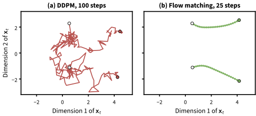
(a) Algorithm 2 adds noise at all but the last of its 100 steps, so its paths are noisy. (b) The Euler sampler of flow matching adds no noise and takes 25 steps (dots) along smooth paths.
Both samplers take steps of equal size in time. However, Elucidating the Design Space of Diffusion-Based Generative Models found that shorter steps near the data and longer ones near the noise give better images, as the errors near the data have a large impact.
And that is all: the full code is in diffusion.py.
Video diffusion and 3D attention
As diffusion moved towards the domain of video, the large amount of data per sample made the compression of latent diffusion even more important, and video models now compress their input in both the spatial and temporal dimensions:
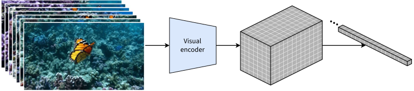
An overview of the latent space compression in Sora. The pre-processing step “turns videos into [visual] patches by first compressing videos into a lower-dimensional latent space and subsequently decomposing the representation into spacetime patches”. Adapted from: Video generation models as world simulators (OpenAI)
Video Attention. A major other challenge with video data is attention: how to correlate image patches across the spatial domain (within a frame), and across the time domain? Given an input of shape \(B \times F \times H \times W \times E\) (batch, number of frames, height and width in patches, and embedding size), we can implement:
- for an attention of shape \(B \times H \times * \times E\), we can do the a spatial attention across patches within a frame \((B * F) \times (H * W) \times E\) followed by a temporal \((B * H * W) \times F \times E\) to attend to the same patch across frames.
- a full 3D attention, where all patches of all frames attend to all others, ie \(B \times F \times H \times W \times E\) into \(B \times (F * H * W) \times E\), which may be an issue because as it leads to a large sequence dimension (of quadratic attention computation).
The following picture illustrates the patches that one patch attends to in each attention:
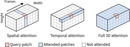
In practice, the spatial and temporal attentions are cheaper and can reuse the spatial layers of a pre-trained image model. The full 3D attention relates every patch to the patches of all frames, which helps to keep objects with large motions consistent across frames, and current video DiTs use it. They encode the position of each patch with a 3D version of the rotary positional embeddings (RoPE): RoPE rotates the queries and keys by the position of their token, and 3D RoPE splits their channels into three groups, rotated by the frame, the row and the column of the patch.
Diffusion vs autoregressive models for video generation
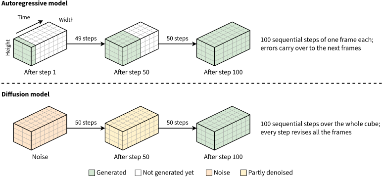
A video is a 3D cube of pixels: height × width × time. An autoregressive model generates a video one frame at a time, each frame conditioned on the previous ones. A diffusion model generates a whole video chunk at once: it starts from a cube of noise and denoises all the frames together over \(T\) steps. The following picture illustrates both:
Both models generate a video of \(F\) frames in a latent space. However, an encoder compresses each frame into a latent of \(d\) values, and a decoder turns each latent back into a frame. So the models only generate a matrix of \(F \times d\) latent values, far fewer than the pixels, as illustrated below:

FLOPs. To count their cost, imagine that both models are only matrix multiplications (matmuls): a stack of layers, each one multiplying its input by a weight matrix of \(d \times d\) values. A matmul \([m \times k] \times [k \times n]\) costs \(2mkn\) FLOPs: a multiply and an accumulate for each of the \(kn\) weights and each of the \(m\) rows of the input. So, in each layer:
- the autoregressive model runs \(F\) sequential steps, one per frame. In each step, it multiplies the latent of one frame, a \(1 \times d\) matrix, by the weights, which costs \(2d^2\) FLOPs, i.e. \(2Fd^2\) FLOPs for the video.
- the diffusion model runs \(T\) sequential steps, one per noise level. In each step, it multiplies the latents of all the frames, an \(F \times d\) matrix, by the weights, which costs \(2Fd^2\) FLOPs, i.e. \(2TFd^2\) FLOPs for the video.
Thus, the diffusion model performs \(T\) times more FLOPs, as it processes all the frames in each of its \(T\) steps, while the autoregressive model processes each frame once. However, both models read the same weights from memory in each step, and a GPU performs hundreds of FLOPs in the time it reads one weight. With 2 FLOPs per weight, the autoregressive model is memory-bound and leaves the GPU mostly idle, as the decode phase of a large language model. The diffusion model uses each weight on the \(F\) frames at once, i.e. \(2F\) FLOPs per weight. So the the diffusion does \(T\) more FLOPs than autoregressive model but benefits from GPU vector computation. On longer videos, its steps fill the GPU and its extra FLOPs take time, but its frames then split across many GPUs (sequence parallelism), while the autoregressive model has a single frame patches per step to split.
Moreover, the diffusion model makes fewer errors. The autoregressive model never revises a frame, so its errors carry over to the next frames and accumulate into flicker and drift, while each diffusion step revises all the frames with the context of the previous and the following ones. However, the autoregressive model can stream its video as it generates frames iteratively, instead of all frames at once. Thus hybrid autoregressive diffusion models (e.g. Diffusion Forcing, CausVid, Self Forcing) perform autoregressive generation of video chunks with diffusion .
Closing Remarks
Sparse Attention. Full 3D attention takes most of the generation time of a video, as its cost grows with the square of the number of patches. However, most attention scores fall on patches that are close in space and time. One solution is Sparse attention. Sliding Tile Attention restricts each tile of patches to a 3D window of neighboring tiles, with tiles of the size of the blocks of FlashAttention, so that the kernel skips whole blocks. Sparse VideoGen finds that each head is either spatial, attending to the patches of nearby frames, or temporal, attending to the same position in all frames, and picks the sparse pattern of each head at runtime. Sparse-Linear Attention, after a short fine-tuning, computes the largest attention weights exactly, approximates most of the others with linear attention, and skips the rest.
Quantization. Quantization stores the weights, and possibly the activations, with fewer bits, improving memory/compute efficiency. SVDQuant quantizes both to 4 bits, so that the matmuls run on 4-bit tensor cores. As 4 bits cannot represent the outliers, it moves the outliers of the activations into the weights, and those of the weights into a low-rank branch, computed with a singular value decomposition (SVD) and kept in 16 bits.
Parallelism. Sequence parallelism splits the patches of a sample across GPUs, with Ulysses or Ring Attention. CFG parallelism runs the conditional and the unconditional passes of classifier-free guidance (CFG) on two GPUs. Both give the exact result of a single GPU, but sequence parallelism communicates in every layer of every step. Diffusion allows a cheaper approximation, as the activations change little from one step to the next. In displaced patch parallelism, each GPU computes its own patches with the activations of the other patches from the previous step, so that the exchange of the new activations overlaps with the compute.
Diffusion language models. Text is discrete, so masked diffusion replaces the Gaussian noise with a mask token. Each reverse step predicts all the masked tokens at once and unmasks some of them, so that one step can generate several tokens. However, the attention is bidirectional, so there is no exact key-value (KV) cache, and each step recomputes the whole sequence. Block diffusion applies the hybrid idea of the video models above to text: it is autoregressive across blocks of tokens, with the finished blocks in a KV cache, and runs diffusion within each block.